Construct amplitude models

\(X\to \pi^-\pi^+\pi^-\)

Model definition: x2pipipi-compass-1391643.json.

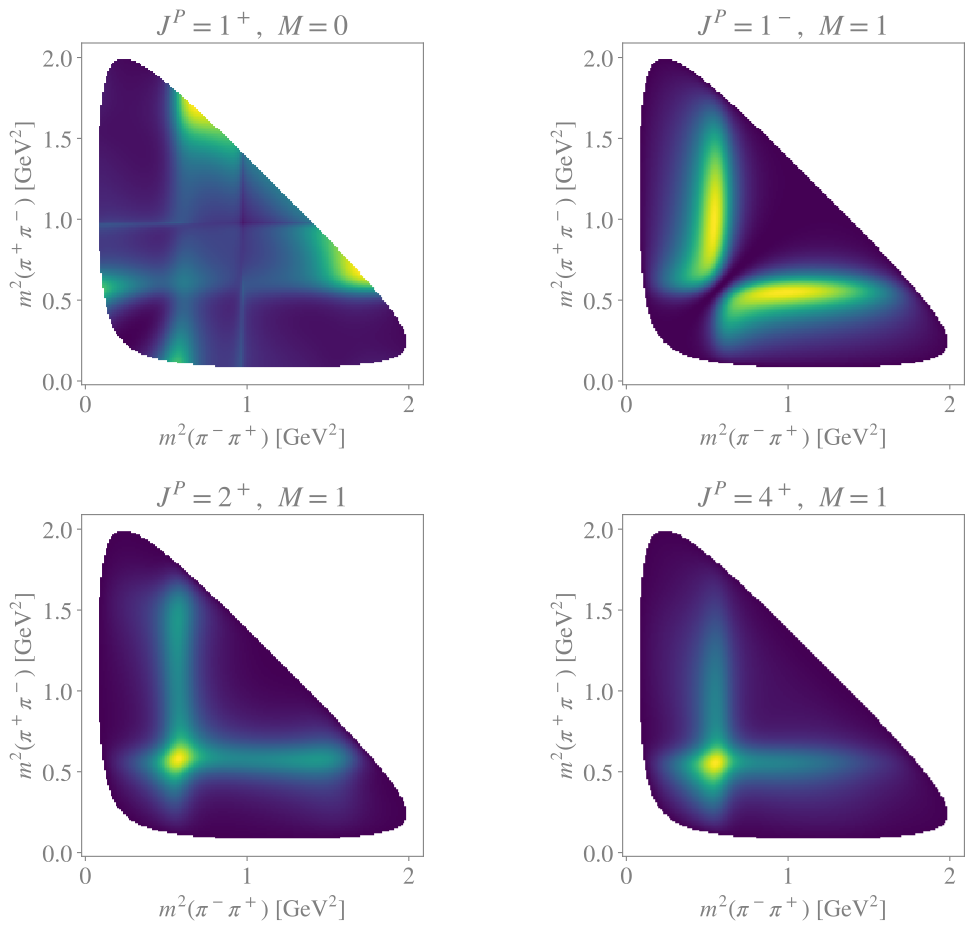
This page demonstrates deserialization and evaluation of a partial-wave analysis of a diffractively produced \(3\pi\) system. The analysis is performed independently in bins of \(3\pi\) mass and transferred momentum. The full analysis contains about 170 decay chains (about 88 waves, symmetrized for the two \(\pi^+\pi^-\) pairs) per bin. See INSPIRE-HEP 1391643 for details.

import logging
from pathlib import Path

import jax.numpy as jnp
import matplotlib.pyplot as plt
import pandas as pd
from ampform_dpd.io.serialization import (
    compile_workspace,
    load_workspace,
    validate_checksums,
)
from matplotlib_inline.backend_inline import set_matplotlib_formats

this_dir = Path(".").absolute()
logging.getLogger("ampform.sympy").setLevel(logging.ERROR)
set_matplotlib_formats("svg")

model_path = this_dir.parent.parent / "models" / "x2pipipi-compass-1391643.json"
workspace = load_workspace(model_path)

The JSON file contains four distributions from the same mass bin. load_workspace formulates all of them, their decays, and their named dynamics functions in one step.

models = workspace.distributions

pd.DataFrame({
    "Distribution": list(models),
    "Decay chains": [len(decay.chains) for decay in workspace.decays.values()],
})

	Distribution	Decay chains
0	compass_3pi_JP=1+_M=0_1540_1560	16
1	compass_3pi_JP=1-_M=1_1540_1560	2
2	compass_3pi_JP=2+_M=1_1540_1560	6
3	compass_3pi_JP=4+_M=1_1540_1560	4

Validation

validate_checksums converts real and complex references, transforms serialized coordinates, and returns one structured result per checkpoint. Failed comparisons or evaluations retain their diagnostics without interrupting the remaining checks.

The status marks 🟢, 🟡, and 🔴 indicate absolute differences of \(<10^{-10}\), \(<10^{-2}\), and \(\ge10^{-2}\), respectively. Failed evaluations are marked 🔴; the diagnostic column provides details.

compiled_workspace = compile_workspace(workspace, backend="jax")
checksum_results = validate_checksums(compiled_workspace)
pd.DataFrame({
    "Distribution": [result.target for result in checksum_results],
    "Point": [result.point_name for result in checksum_results],
    "Reference": [result.reference for result in checksum_results],
    "Computed": [result.value for result in checksum_results],
    "Difference": [result.difference for result in checksum_results],
    "Status": [
        "🟢" if result.difference < 1e-10 else "🟡" if result.difference < 1e-2 else "🔴"
        for result in checksum_results
    ],
    "Diagnostic": [result.diagnostic for result in checksum_results],
})

	Distribution	Point	Reference	Computed	Difference	Status	Diagnostic
0	compass_3pi_JP=1+_M=0_1540_1560	validation_point1	0.557753+0.000000j	0.557753+0.000000j	1.321165e-14	🟢	None
1	compass_3pi_JP=1+_M=0_1540_1560	validation_point2	1.436252+0.000000j	1.436252+0.000000j	2.420286e-14	🟢	None
2	compass_3pi_JP=1+_M=0_1540_1560	validation_point3	0.108395+0.000000j	0.108395+0.000000j	4.579670e-16	🟢	None
3	compass_3pi_JP=1+_M=0_1540_1560	validation_point4	0.791847+0.000000j	0.791847+0.000000j	9.992007e-15	🟢	None
4	compass_3pi_JP=1-_M=1_1540_1560	validation_point1	0.045205+0.000000j	0.045205+0.000000j	4.718448e-16	🟢	None
5	compass_3pi_JP=1-_M=1_1540_1560	validation_point2	0.010651+0.000000j	0.010651+0.000000j	1.214306e-16	🟢	None
6	compass_3pi_JP=1-_M=1_1540_1560	validation_point3	0.018570+0.000000j	0.018570+0.000000j	1.734723e-16	🟢	None
7	compass_3pi_JP=1-_M=1_1540_1560	validation_point4	0.090084+0.000000j	0.090084+0.000000j	8.881784e-16	🟢	None
8	compass_3pi_JP=2+_M=1_1540_1560	validation_point1	0.017082+0.000000j	0.017082-0.000000j	3.825906e-17	🟢	None
9	compass_3pi_JP=2+_M=1_1540_1560	validation_point2	0.057953+0.000000j	0.057953+0.000000j	1.228281e-15	🟢	None
10	compass_3pi_JP=2+_M=1_1540_1560	validation_point3	0.035384+0.000000j	0.035384-0.000000j	2.462156e-16	🟢	None
11	compass_3pi_JP=2+_M=1_1540_1560	validation_point4	0.112218+0.000000j	0.112218-0.000000j	1.720854e-15	🟢	None
12	compass_3pi_JP=4+_M=1_1540_1560	validation_point1	0.020556+0.000000j	0.020556+0.000000j	5.412337e-16	🟢	None
13	compass_3pi_JP=4+_M=1_1540_1560	validation_point2	0.011818+0.000000j	0.011818+0.000000j	1.908196e-17	🟢	None
14	compass_3pi_JP=4+_M=1_1540_1560	validation_point3	0.017550+0.000000j	0.017550+0.000000j	1.110223e-16	🟢	None
15	compass_3pi_JP=4+_M=1_1540_1560	validation_point4	0.105833+0.000000j	0.105833+0.000000j	8.049117e-16	🟢	None
16	R(1274)	validation_point_m12sq	1.682682+0.620869j	1.682682+0.620869j	1.493652e-15	🟢	None
17	R(1690)	validation_point_m12sq	0.564308+0.103183j	0.564308+0.103183j	1.241267e-16	🟢	None
18	R(600)	validation_point_m12sq	0.101724+1.027344j	0.101724+1.027344j	2.423651e-16	🟢	None
19	R(768)	validation_point_m12sq	-1.732183+0.632399j	-1.732183+0.632399j	3.155847e-15	🟢	None
20	R(965)	validation_point_m12sq	-0.921258+2.147040j	-0.921258+2.147040j	1.938921e-15	🟢	None

Visualization

Dalitz plots

The four distributions in the selected \(3\pi\) mass bin are shown over the same pair of Mandelstam variables.

x_subsystem, y_subsystem = 3, 1
resolution = 200
intensity_grids = {}
for name, model in models.items():
    masses = sorted(model.masses, key=str)

    def invariant_limits(subsystem: int) -> tuple[float, float]:
        a, b = sorted({1, 2, 3} - {subsystem})
        minimum = (masses[a] + masses[b]) ** 2
        maximum = (masses[0] - masses[subsystem]) ** 2
        return (
            float(minimum.xreplace(model.masses)),
            float(maximum.xreplace(model.masses)),
        )

    x_min, x_max = invariant_limits(x_subsystem)
    y_min, y_max = invariant_limits(y_subsystem)
    x_margin = 0.05 * (x_max - x_min)
    y_margin = 0.05 * (y_max - y_min)
    x, y = jnp.meshgrid(
        jnp.linspace(x_min - x_margin, x_max + x_margin, resolution),
        jnp.linspace(y_min - y_margin, y_max + y_margin, resolution),
    )
    function = compiled_workspace.functions[name]
    values = jnp.real(
        function({f"sigma{x_subsystem}": x, f"sigma{y_subsystem}": y})
    )
    intensity_grids[name] = (x, y, values / jnp.nansum(values))

# cspell:ignore bbox edgecolor facecolor fontset fontsize labelcolor mathtext ncol
# cspell:ignore hspace savefig sharey STIX wspace xtick ytick
plt.rcParams.update({
    "axes.edgecolor": "#808080",
    "axes.facecolor": "none",
    "axes.labelcolor": "#808080",
    "figure.facecolor": "none",
    "font.family": "serif",
    "font.serif": ["STIXGeneral", "DejaVu Serif"],
    "font.size": 18,
    "mathtext.fontset": "stix",
    "savefig.transparent": True,
    "text.color": "#808080",
    "xtick.color": "#808080",
    "ytick.color": "#808080",
})

subplot_titles = {
    "compass_3pi_JP=1+_M=0_1540_1560": R"$J^P=1^+,\ M=0$",
    "compass_3pi_JP=1-_M=1_1540_1560": R"$J^P=1^-,\ M=1$",
    "compass_3pi_JP=2+_M=1_1540_1560": R"$J^P=2^+,\ M=1$",
    "compass_3pi_JP=4+_M=1_1540_1560": R"$J^P=4^+,\ M=1$",
}
fig, axes = plt.subplots(2, 2, figsize=(14, 11))
for ax, (name, (x, y, values)) in zip(axes.flat, intensity_grids.items(), strict=True):
    ax.pcolormesh(x, y, values, rasterized=True)
    ax.set_aspect("equal")
    ax.set_title(subplot_titles[name])
    ax.set_xlabel(R"$m^2(\pi^-\pi^+)$ [GeV$^2$]")
    ax.set_ylabel(R"$m^2(\pi^+\pi^-)$ [GeV$^2$]")
fig.subplots_adjust(hspace=0.38, wspace=0.08)
plt.show()