Construct three-body decay

\(\Lambda_c^+ \to p K^- \pi^+\)

Model definition: lc2ppik-lhcb-2683025.json.

This notebook illustrates the use of the ampform_dpd.io.serialization module for the decay \(\Lambda_c^+ \to p K^- \pi^+\). The corresponding model was optimized to a data sample of roughly half a million \(\Lambda_c^{\pm}\) decay candidates by the LHCb collaboration, INSPIRE-HEP 2683025.

Warning

The ampform_dpd.io.serialization module is a preview feature. This notebook illustrates the complete workflow for loading the amplitude model JSON file into a symbolic workspace, compiling it, and validating its serialized checksums.

Import model

Import Python libraries
import logging
from pathlib import Path

import jax.numpy as jnp
import matplotlib.pyplot as plt
import pandas as pd
import sympy as sp
from ampform.dynamics.form_factor import FormFactor
from ampform_dpd.decay import FinalStateID, State, ThreeBodyDecay
from ampform_dpd.dynamics import (
    BreitWigner,
    ChannelArguments,
    MultichannelBreitWigner,
)
from ampform_dpd.io import (
    aslatex,
    simplify_latex_rendering,
    unfold_definitions,
)
from ampform_dpd.io.serialization import (
    compile_workspace,
    load_workspace,
    validate_checksums,
)
from ampform_dpd.io.serialization.amplitude import (
    HelicityRecoupling,
    LSRecoupling,
    ParityRecoupling,
    formulate_aligned_amplitude,
    formulate_chain_amplitude,
    formulate_recoupling,
)
from ampform_dpd.io.serialization.dynamics import (
    formulate_breit_wigner,
    formulate_dynamics,
    formulate_form_factor,
    formulate_multichannel_breit_wigner,
)
from ampform_dpd.io.serialization.format import (
    get_decay_chains,
    get_function_definition,
)
from IPython.display import JSON, Math
from matplotlib_inline.backend_inline import set_matplotlib_formats
from mpl_toolkits.axes_grid1 import make_axes_locatable  # cspell:ignore mpl_toolkits
from tqdm.auto import tqdm

this_dir = Path(".").absolute()
logging.getLogger("ampform.sympy").setLevel(logging.ERROR)
simplify_latex_rendering()
set_matplotlib_formats("svg")
model_path = this_dir.parent.parent / "models" / "lc2ppik-lhcb-2683025.json"
Name-to-LaTeX converter
def to_latex(name: str) -> str:
    latex = {
        "Lc": R"\Lambda_c^+",
        "pi": R"\pi^+",
        "K": "K^-",
        "p": "p",
    }.get(name)
    if latex is not None:
        return latex
    mass_str = name[1:].strip("(").strip(")")
    subsystem_letter = name[0]
    subsystem = {"D": "D", "K": "K", "L": R"\Lambda"}.get(subsystem_letter)
    if subsystem is None:
        return name
    return f"{subsystem}({mass_str})"
workspace = load_workspace(model_path, to_latex=to_latex)
model_definition = workspace.definition
((intensity_name, decay),) = workspace.decays.items()
Math(aslatex(decay, with_jp=True))

\(\displaystyle \begin{array}{c} \Lambda_c^+\left[J=\frac{1}{2}\right] \to \left(D(1232)\left[J=\frac{3}{2}\right] \to p\left[J=\frac{1}{2}\right] \pi^+\left[J=0\right]\right) K^-\left[J=0\right] \\ \Lambda_c^+\left[J=\frac{1}{2}\right] \to \left(D(1600)\left[J=\frac{3}{2}\right] \to p\left[J=\frac{1}{2}\right] \pi^+\left[J=0\right]\right) K^-\left[J=0\right] \\ \Lambda_c^+\left[J=\frac{1}{2}\right] \to \left(D(1700)\left[J=\frac{3}{2}\right] \to p\left[J=\frac{1}{2}\right] \pi^+\left[J=0\right]\right) K^-\left[J=0\right] \\ \Lambda_c^+\left[J=\frac{1}{2}\right] \to \left(K(1430)\left[J=0\right] \to \pi^+\left[J=0\right] K^-\left[J=0\right]\right) p\left[J=\frac{1}{2}\right] \\ \Lambda_c^+\left[J=\frac{1}{2}\right] \to \left(K(700)\left[J=0\right] \to \pi^+\left[J=0\right] K^-\left[J=0\right]\right) p\left[J=\frac{1}{2}\right] \\ \Lambda_c^+\left[J=\frac{1}{2}\right] \to \left(K(892)\left[J=1\right] \to \pi^+\left[J=0\right] K^-\left[J=0\right]\right) p\left[J=\frac{1}{2}\right] \\ \Lambda_c^+\left[J=\frac{1}{2}\right] \to \left(\Lambda(1405)\left[J=\frac{1}{2}\right] \to K^-\left[J=0\right] p\left[J=\frac{1}{2}\right]\right) \pi^+\left[J=0\right] \\ \Lambda_c^+\left[J=\frac{1}{2}\right] \to \left(\Lambda(1520)\left[J=\frac{3}{2}\right] \to K^-\left[J=0\right] p\left[J=\frac{1}{2}\right]\right) \pi^+\left[J=0\right] \\ \Lambda_c^+\left[J=\frac{1}{2}\right] \to \left(\Lambda(1600)\left[J=\frac{1}{2}\right] \to K^-\left[J=0\right] p\left[J=\frac{1}{2}\right]\right) \pi^+\left[J=0\right] \\ \Lambda_c^+\left[J=\frac{1}{2}\right] \to \left(\Lambda(1670)\left[J=\frac{1}{2}\right] \to K^-\left[J=0\right] p\left[J=\frac{1}{2}\right]\right) \pi^+\left[J=0\right] \\ \Lambda_c^+\left[J=\frac{1}{2}\right] \to \left(\Lambda(1690)\left[J=\frac{3}{2}\right] \to K^-\left[J=0\right] p\left[J=\frac{1}{2}\right]\right) \pi^+\left[J=0\right] \\ \Lambda_c^+\left[J=\frac{1}{2}\right] \to \left(\Lambda(2000)\left[J=\frac{1}{2}\right] \to K^-\left[J=0\right] p\left[J=\frac{1}{2}\right]\right) \pi^+\left[J=0\right] \\ \end{array}\)

Dynamics

See also RUB-EP1/amplitude-serialization#22 about serialization of custom lineshapes.

chain_defs = get_decay_chains(model_definition)

Vertices

Blatt-Weisskopf form factor

Code
s, m1, m2, angular_momentum, d = sp.symbols("s m1 m2 L R", nonnegative=True)
expr = FormFactor(s, m1, m2, angular_momentum, d)
Math(aslatex(unfold_definitions(expr)))

\(\displaystyle \begin{aligned} \mathcal{F}_{L}\left(s, m_{1}, m_{2}\right) \;&=\; \sqrt{B_{L}^2\left(R^{2} q^2\left(s\right)\right)} \\ B_{L}^2\left(R^{2} q^2\left(s\right)\right) \;&=\; \frac{\left|{h_{L}^{(1)}\left(1\right)}\right|^{2}}{R^{2} \left|{h_{L}^{(1)}\left(R \sqrt{q^2\left(s\right)}\right)}\right|^{2} q^2\left(s\right)} \\ q^2\left(s\right) \;&=\; \frac{\left(s - \left(m_{1} - m_{2}\right)^{2}\right) \left(s - \left(m_{1} + m_{2}\right)^{2}\right)}{4 s} \\ h_{L}^{(1)}\left(z\right) \;&=\; \frac{\left(- i\right)^{L + 1} e^{i z} \sum_{k=0}^{L} \frac{\left(\frac{i}{2 z}\right)^{k} \left(k + L\right)!}{k! \left(- k + L\right)!}}{z} \\ \end{aligned}\)

ff_l1520 = formulate_form_factor(
    vertex=chain_defs[2]["vertices"][0],
    model=model_definition,
)
Math(aslatex(ff_l1520))

\(\displaystyle \begin{array}{rcl} \frac{\sqrt{2} \mathcal{F}_{1}\left(m_{0}^{2}, \sqrt{\sigma_{2}}, m_{2}\right)}{2} \\ R_{Lc} &=& 5.0 \\ \end{array}\)

Propagators

Breit-Wigner

Code
s, m0, gamma0, m1, m2, angular_momentum, d = sp.symbols("s m0 Gamma0 m1 m2 L R", nonnegative=True)
expr = BreitWigner(s, m0, gamma0, m1, m2, angular_momentum, d)
Math(aslatex(unfold_definitions(expr)))

\(\displaystyle \begin{aligned} \mathcal{R}^\mathrm{BW}_{L}\left(s; m_{0}, \Gamma_{0}\right) \;&=\; \mathcal{R}^\mathrm{BW}\left(s; m_{0}, \Gamma_{0}\left(s\right)\right) \\ \mathcal{R}^\mathrm{BW}\left(s; m_{0}, \Gamma_{0}\left(s\right)\right) \;&=\; \frac{1}{m_{0}^{2} - i m_{0} \Gamma_{0}\left(s\right) - s} \\ \Gamma_{0}\left(s\right) \;&=\; \frac{\Gamma_{0} \mathcal{F}_{L}\left(s, m_{1}, m_{2}\right)^{2} \rho\left(s\right)}{\mathcal{F}_{L}\left(m_{0}^{2}, m_{1}, m_{2}\right)^{2} \rho_{0}\left(m_{0}^{2}\right)} \\ \mathcal{F}_{L}\left(s, m_{1}, m_{2}\right) \;&=\; \sqrt{B_{L}^2\left(R^{2} q^2\left(s\right)\right)} \\ \rho\left(s\right) \;&=\; \frac{\sqrt{\left(s - \left(m_{1} - m_{2}\right)^{2}\right) \left(s - \left(m_{1} + m_{2}\right)^{2}\right)}}{s} \\ B_{L}^2\left(R^{2} q^2\left(s\right)\right) \;&=\; \frac{\left|{h_{L}^{(1)}\left(1\right)}\right|^{2}}{R^{2} \left|{h_{L}^{(1)}\left(R \sqrt{q^2\left(s\right)}\right)}\right|^{2} q^2\left(s\right)} \\ q^2\left(s\right) \;&=\; \frac{\left(s - \left(m_{1} - m_{2}\right)^{2}\right) \left(s - \left(m_{1} + m_{2}\right)^{2}\right)}{4 s} \\ h_{L}^{(1)}\left(z\right) \;&=\; \frac{\left(- i\right)^{L + 1} e^{i z} \sum_{k=0}^{L} \frac{\left(\frac{i}{2 z}\right)^{k} \left(k + L\right)!}{k! \left(- k + L\right)!}}{z} \\ \end{aligned}\)

k892_bw = formulate_breit_wigner(
    propagator=chain_defs[20]["propagators"][0],
    resonance=to_latex(chain_defs[20]["name"]),
    model=model_definition,
)
Math(aslatex(k892_bw))

\(\displaystyle \begin{array}{rcl} \mathcal{R}^\mathrm{BW}_{L=1}\left(\sigma_{1}; m_{K(892)}, \Gamma_{K(892)}\right) &=& \mathcal{R}^\mathrm{BW}\left(\sigma_{1}; m_{K(892)}, \Gamma_{892}\left(\sigma_{1}\right)\right) \\ m_{K(892)} &=& 0.8955 \\ \Gamma_{K(892)} &=& 0.047299999999999995 \\ m_{2} &=& 0.13957018 \\ m_{3} &=& 0.493677 \\ R_\mathrm{res} &=& 1.5 \\ \end{array}\)

Multi-channel Breit-Wigner

The gsq value that is serialized for each channel is the coupling squared, not an energy width. The channel term \(\Gamma^\text{ch}\) below follows the same convention as HadronicLineshapes.jl. See ComPWA/ampform-dpd#199.

Code
s, m0, m1, m2, angular_momentum, d = sp.symbols("s m0 m1 m2 L R", nonnegative=True)
channels = tuple(
    ChannelArguments(
        s,
        m0,
        coupling_squared=sp.Symbol(f"g_{{{i}}}^2", nonnegative=True),
        m1=sp.Symbol(f"m_{{a,{i}}}", nonnegative=True),
        m2=sp.Symbol(f"m_{{b,{i}}}", nonnegative=True),
        angular_momentum=sp.Symbol(f"L{i}", integer=True, nonnegative=True),
        meson_radius=d,
    )
    for i in [1, 2]
)
expr = MultichannelBreitWigner(s, m0, channels)
Math(aslatex(unfold_definitions(expr)))

\(\displaystyle \begin{aligned} \mathcal{R}^\mathrm{BW}_\mathrm{multi}\left(s; g_{1}^2, g_{2}^2\right) \;&=\; \mathcal{R}^\mathrm{BW}_{L=0}\left(s; m_{0}, \Gamma^\text{ch}\left(s; m_{0}, g_{1}^2\right) + \Gamma^\text{ch}\left(s; m_{0}, g_{2}^2\right)\right) \\ \mathcal{R}^\mathrm{BW}_{L=0}\left(s; m_{0}, \Gamma^\text{ch}\left(s; m_{0}, g_{1}^2\right) + \Gamma^\text{ch}\left(s; m_{0}, g_{2}^2\right)\right) \;&=\; \frac{1}{m_{0}^{2} - i m_{0} \left(\Gamma^\text{ch}\left(s; m_{0}, g_{1}^2\right) + \Gamma^\text{ch}\left(s; m_{0}, g_{2}^2\right)\right) - s} \\ \Gamma^\text{ch}\left(s; m_{0}, g_{1}^2\right) \;&=\; \frac{g_{1}^2 \mathcal{F}_{L_{1}}\left(s, m_{a,1}, m_{b,1}\right)^{2} \rho\left(s\right)}{m_{0}} \\ \mathcal{F}_{L_{1}}\left(s, m_{a,1}, m_{b,1}\right) \;&=\; \sqrt{B_{L_{1}}^2\left(R^{2} q^2\left(s\right)\right)} \\ \rho\left(s\right) \;&=\; \frac{\sqrt{\left(s - \left(m_{a,1} - m_{b,1}\right)^{2}\right) \left(s - \left(m_{a,1} + m_{b,1}\right)^{2}\right)}}{s} \\ B_{L_{1}}^2\left(R^{2} q^2\left(s\right)\right) \;&=\; \frac{\left|{h_{L_{1}}^{(1)}\left(1\right)}\right|^{2}}{R^{2} \left|{h_{L_{1}}^{(1)}\left(R \sqrt{q^2\left(s\right)}\right)}\right|^{2} q^2\left(s\right)} \\ q^2\left(s\right) \;&=\; \frac{\left(s - \left(m_{a,1} - m_{b,1}\right)^{2}\right) \left(s - \left(m_{a,1} + m_{b,1}\right)^{2}\right)}{4 s} \\ h_{L_{1}}^{(1)}\left(z\right) \;&=\; \frac{\left(- i\right)^{L_{1} + 1} e^{i z} \sum_{k=0}^{L_{1}} \frac{\left(\frac{i}{2 z}\right)^{k} \left(k + L_{1}\right)!}{k! \left(- k + L_{1}\right)!}}{z} \\ \end{aligned}\)
l1405_flatte = formulate_multichannel_breit_wigner(
    propagator=chain_defs[0]["propagators"][0],
    resonance=to_latex(chain_defs[0]["name"]),
    model=model_definition,
)
Math(aslatex(l1405_flatte))

\(\displaystyle \begin{array}{rcl} \frac{1}{m_{\Lambda(1405)}^{2} - \sigma_{2} - i \left(\Gamma_{\Lambda(1405)} \mathcal{F}_{0}\left(\sigma_{2}, m_{3}, m_{1}\right)^{2} \rho^\mathrm{c}_{2}\left(\sigma_{2}\right) + \Gamma_{\Lambda(1405)}^\text{ch. 2} \mathcal{F}_{0}\left(\sigma_{2}, m_{a,2}, m_{b,2}\right)^{2} \rho^\mathrm{c}_{2}\left(\sigma_{2}\right)\right)} \\ m_{\Lambda(1405)} &=& 1.4051 \\ \Gamma_{\Lambda(1405)} &=& 0.328725260215546 \\ m_{3} &=& 0.938272046 \\ m_{1} &=& 0.493677 \\ R_{\Lambda(1405)} &=& 0 \\ m_{a,2} &=& 1.18937 \\ m_{b,2} &=& 0.13957018 \\ \Gamma_{\Lambda(1405)}^\text{ch. 2} &=& 0.328725260215546 \\ \end{array}\)

Breit-Wigner with exponential

The Bugg lineshapes are serialized as generic_function expression strings. The built-in dynamics builder parses these expressions and substitutes \(i\) and \(\sigma\) with the imaginary unit and the Mandelstam variable of the propagator node, respectively.

get_function_definition("K700_BuggBW", model_definition)
mappingproxy({'name': 'K700_BuggBW',
              'type': 'generic_function',
              'expression': '1/(0.824^2 - σ - i * 0.824 * (σ - 0.23397706275638377) / (0.824^2 - 0.23397706275638377) * 0.478 * exp(-0.941060 * σ))'})
k700_bugg_bw = formulate_dynamics(chain_defs[18], model_definition, to_latex)
Math(aslatex(k700_bugg_bw))

\(\displaystyle \begin{array}{rcl} \frac{1}{- \sigma_{1} - 0.88510773180649964 i \left(\sigma_{1} - 0.23397706275638377\right) e^{- 0.94106 \sigma_{1}} + 0.678976} \\ \end{array}\)

Construct amplitude model

Unpolarized intensity

λ0, λ1, λ2, λ3 = sp.symbols("lambda(:4)", rational=True)
amplitude_expr, _ = formulate_aligned_amplitude(model_definition, λ0, λ1, λ2, λ3)
amplitude_expr.cleanup()

\(\displaystyle \sum_{\lambda_0^{\prime}=-1/2}^{1/2} \sum_{\lambda_1^{\prime}=-1/2}^{1/2}{A^{1}_{\lambda_0^{\prime}, \lambda_1^{\prime}, 0, 0} d^{\frac{1}{2}}_{\lambda_1^{\prime},\lambda_{1}}\left(\zeta^1_{1(1)}\right) d^{\frac{1}{2}}_{\lambda_{0},\lambda_0^{\prime}}\left(\zeta^0_{1(1)}\right) + A^{2}_{\lambda_0^{\prime}, \lambda_1^{\prime}, 0, 0} d^{\frac{1}{2}}_{\lambda_1^{\prime},\lambda_{1}}\left(\zeta^1_{2(1)}\right) d^{\frac{1}{2}}_{\lambda_{0},\lambda_0^{\prime}}\left(\zeta^0_{2(1)}\right) + A^{3}_{\lambda_0^{\prime}, \lambda_1^{\prime}, 0, 0} d^{\frac{1}{2}}_{\lambda_1^{\prime},\lambda_{1}}\left(\zeta^1_{3(1)}\right) d^{\frac{1}{2}}_{\lambda_{0},\lambda_0^{\prime}}\left(\zeta^0_{3(1)}\right)}\)

The workspace formulates every serialized distribution while it is loaded. The full intensity model is therefore available without another formulation step.

model = workspace.distributions[intensity_name]

Amplitude for the decay chain

Helicity recouplings

Code
λa = sp.Symbol(R"\lambda_a", rational=True)
λb = sp.Symbol(R"\lambda_b", rational=True)
λa0 = sp.Symbol(R"\lambda_a^0", rational=True)
λb0 = sp.Symbol(R"\lambda_b^0", rational=True)
f = sp.Symbol("f", integer=True)
l = sp.Symbol("l", integer=True, nonnegative=True)
s = sp.Symbol("s", nonnegative=True, rational=True)
ja = sp.Symbol("j_a", nonnegative=True, rational=True)
jb = sp.Symbol("j_b", nonnegative=True, rational=True)
j = sp.Symbol("j", nonnegative=True, rational=True)
exprs = [
    HelicityRecoupling(λa, λb, λa0, λb0),
    ParityRecoupling(λa, λb, λa0, λb0, f),
    LSRecoupling(λa, λb, l, s, ja, jb, j),
]
Math(aslatex({e: e.doit(deep=False) for e in exprs}))

\(\displaystyle \begin{aligned} \mathcal{H}^\text{helicity}\left(\lambda_{a},\lambda_{b}\middle|\lambda^{0}_{a},\lambda^{0}_{b}\right) \;&=\; \delta_{\lambda_{a} \lambda^{0}_{a}} \delta_{\lambda_{b} \lambda^{0}_{b}} \\ \mathcal{H}^\text{parity}\left(\lambda_{a},\lambda_{b}\middle|\lambda^{0}_{a},\lambda^{0}_{b},f\right) \;&=\; f \delta_{\lambda_{a}, - \lambda^{0}_{a}} \delta_{\lambda_{b}, - \lambda^{0}_{b}} + \delta_{\lambda_{a} \lambda^{0}_{a}} \delta_{\lambda_{b} \lambda^{0}_{b}} \\ \mathcal{H}^\text{parity}\left(\lambda_{a},\lambda_{b}\middle|l,s,j_{a},j_{b},j\right) \;&=\; \frac{\sqrt{2 l + 1} C^{s,\lambda_{a} - \lambda_{b}}_{j_{a},\lambda_{a},j_{b},- \lambda_{b}} C^{j,\lambda_{a} - \lambda_{b}}_{l,0,s,\lambda_{a} - \lambda_{b}}}{\sqrt{2 j + 1}} \\ \end{aligned}\)

Recoupling deserialization

Code
recouplings = [
    formulate_recoupling(model_definition, chain_idx=0, vertex_idx=i) for i in range(2)
]
Math(aslatex({e: e.doit(deep=False) for e in recouplings}))

\(\displaystyle \begin{aligned} \mathcal{H}^\text{helicity}\left(\lambda_{R},\lambda_{2}\middle|\frac{1}{2},0\right) \;&=\; \delta_{0 \lambda_{2}} \delta_{\frac{1}{2} \lambda_{R}} \\ \mathcal{H}^\text{parity}\left(\lambda_{3},\lambda_{1}\middle|0,\frac{1}{2},1\right) \;&=\; \delta_{- \frac{1}{2} \lambda_{1}} \delta_{0 \lambda_{3}} + \delta_{0 \lambda_{3}} \delta_{\frac{1}{2} \lambda_{1}} \\ \end{aligned}\)

Chain amplitudes

definitions = formulate_chain_amplitude(λ0, λ1, λ2, λ3, model_definition, chain_idx=0)
Math(aslatex(definitions))

\(\displaystyle \begin{aligned} A^{2}_{\lambda_{0}, \lambda_{1}, \lambda_{2}, \lambda_{3}} \;&=\; \sum_{\lambda_{R}=-1/2}^{1/2}{\frac{\left(-1\right)^{- \lambda_{2}} \left(-1\right)^{\frac{1}{2} - \lambda_{1}} \sqrt{2} c^{L1405[1/2]}_{\frac{1}{2}, 0, 0} \delta_{\lambda_{0}, \lambda_{R} - \lambda_{2}} \mathcal{H}^\text{helicity}\left(\lambda_{R},\lambda_{2}\middle|\frac{1}{2},0\right) \mathcal{H}^\text{parity}\left(\lambda_{3},\lambda_{1}\middle|0,\frac{1}{2},1\right) d^{\frac{1}{2}}_{\lambda_{R},- \lambda_{1} + \lambda_{3}}\left(\theta_{31}\right)}{m_{L1405}^{2} - \sigma_{2} - i \left(\Gamma_{L1405} \mathcal{F}_{0}\left(\sigma_{2}, m_{3}, m_{1}\right)^{2} \rho^\mathrm{c}_{2}\left(\sigma_{2}\right) + \Gamma_{L1405}^\text{ch. 2} \mathcal{F}_{0}\left(\sigma_{2}, m_{a,2}, m_{b,2}\right)^{2} \rho^\mathrm{c}_{2}\left(\sigma_{2}\right)\right)}} \\ c^{L1405[1/2]}_{\frac{1}{2}, 0, 0} \;&=\; 7.38649400481717+1.971018433257411i \\ m_{L1405} \;&=\; 1.4051 \\ \Gamma_{L1405} \;&=\; 0.328725260215546 \\ m_{3} \;&=\; 0.938272046 \\ m_{1} \;&=\; 0.493677 \\ R_{L1405} \;&=\; 0 \\ m_{a,2} \;&=\; 1.18937 \\ m_{b,2} \;&=\; 0.13957018 \\ \Gamma_{L1405}^\text{ch. 2} \;&=\; 0.328725260215546 \\ \theta_{31} \;&=\; \operatorname{acos}{\left(\frac{2 \sigma_{2} \left(- m_{2}^{2} - m_{3}^{2} + \sigma_{1}\right) - \left(m_{0}^{2} - m_{2}^{2} - \sigma_{2}\right) \left(- m_{1}^{2} + m_{3}^{2} + \sigma_{2}\right)}{\sqrt{\lambda\left(m_{0}^{2}, m_{2}^{2}, \sigma_{2}\right)} \sqrt{\lambda\left(\sigma_{2}, m_{3}^{2}, m_{1}^{2}\right)}} \right)} \\ \end{aligned}\)

Validation

compile_workspace turns the symbolic workspace into numerical TensorWaves functions. Its default targets are the distributions and named functions referenced by the serialized checksums. validate_checksums transforms each reference point to the required coordinates and returns a structured result without aborting the other checks when an individual evaluation fails.

The status marks 🟢, 🟡, and 🔴 indicate absolute differences of \(<10^{-10}\), \(<10^{-2}\), and \(\ge10^{-2}\), respectively. Failed evaluations are marked 🔴; the diagnostic column provides details. The diagnostic column is hidden when all statuses are 🟢.

Compile and validate all checksum targets
compiled_workspace = compile_workspace(workspace, backend="jax")
checksum_results = validate_checksums(compiled_workspace)
validation_table = pd.DataFrame({
    "Distribution": [result.target for result in checksum_results],
    "Point": [result.point_name for result in checksum_results],
    "Computed": [result.value for result in checksum_results],
    "Expected": [result.reference for result in checksum_results],
    "Difference": [result.difference for result in checksum_results],
    "Status": [
        "🟢" if result.difference < 1e-10 else "🟡" if result.difference < 1e-2 else "🔴"
        for result in checksum_results
    ],
    "Diagnostic": [result.diagnostic for result in checksum_results],
})
if validation_table["Status"].eq("🟢").all():
    validation_table = validation_table.drop(columns="Diagnostic")
assert all(result.passed for result in checksum_results)
validation_table
Distribution Point Computed Expected Difference Status
0 default_model validation_point 9345.853381+   0.000000j 9345.853381+   0.000000j 9.094947e-12 🟢
1 L1405_Flatte validation_point_m31sq -0.748060+   0.225214j -0.748060+   0.225214j 1.665335e-16 🟢
2 L1690_BW validation_point_m31sq -1.856393+   1.397092j -1.856393+   1.397092j 2.452563e-15 🟢
3 D1232_BW validation_point_m12sq -0.375591+   0.286720j -0.375591+   0.286720j 8.617648e-16 🟢
4 L1520_BW validation_point_m31sq -0.651903+   0.551371j -0.651903+   0.551371j 1.350645e-15 🟢
5 L1600_BW validation_point_m31sq -0.571161+   0.851729j -0.571161+   0.851729j 4.965068e-16 🟢
6 L2000_BW validation_point_m31sq 1.139903+   0.463291j 1.139903+   0.463291j 5.236912e-16 🟢
7 D1600_BW validation_point_m12sq -0.754261+   0.953349j -0.754261+   0.953349j 1.790181e-15 🟢
8 D1700_BW validation_point_m12sq -0.324205+   0.915217j -0.324205+   0.915217j 5.357905e-15 🟢
9 K892_BW validation_point_m23sq -1.616042+   0.300764j -1.616042+   0.300764j 7.021667e-16 🟢
10 L1670_BW validation_point_m31sq -2.383990+   0.340064j -2.383990+   0.340064j 4.440892e-16 🟢

Visualization

Configure the visualizations
i, j = 2, 1
k, *_ = {1, 2, 3} - {i, j}
resolution = 1_000
masses = sorted(model.masses, key=str)
x_min = float(((masses[j] + masses[k]) ** 2).xreplace(model.masses))
x_max = float(((masses[0] - masses[i]) ** 2).xreplace(model.masses))
y_min = float(((masses[i] + masses[k]) ** 2).xreplace(model.masses))
y_max = float(((masses[0] - masses[j]) ** 2).xreplace(model.masses))
x_margin = 0.05 * (x_max - x_min)
y_margin = 0.05 * (y_max - y_min)
x, y = jnp.meshgrid(
    jnp.linspace(x_min - x_margin, x_max + x_margin, num=resolution),
    jnp.linspace(y_min - y_margin, y_max + y_margin, num=resolution),
)
dalitz_data = {f"sigma{i}": x, f"sigma{j}": y}
intensity_function = compiled_workspace.functions[intensity_name]
intensities = intensity_function(dalitz_data)
normalized_intensities = intensities / jnp.nansum(intensities)


def get_decay_products(
    decay: ThreeBodyDecay,
    subsystem: FinalStateID,
) -> tuple[State, State]:
    return tuple(s for s in decay.final_state.values() if s.index != subsystem)


sigma_labels = {
    subsystem: Rf"$\sigma_{subsystem} = M^2\left({' '.join(p.latex for p in get_decay_products(decay, subsystem))}\right)$"
    for subsystem in (1, 2, 3)
}
# cspell:ignore bbox edgecolor facecolor fontset fontsize labelcolor mathtext ncol savefig
# cspell:ignore sharey startswith STIX wspace xtick ytick
plt.rcParams.update({
    "axes.edgecolor": "#808080",
    "axes.facecolor": "none",
    "axes.labelcolor": "#808080",
    "figure.facecolor": "none",
    "font.family": "serif",
    "font.serif": ["STIXGeneral", "DejaVu Serif"],
    "font.size": 18,
    "mathtext.fontset": "stix",
    "savefig.transparent": True,
    "text.color": "#808080",
    "xtick.color": "#808080",
    "ytick.color": "#808080",
})
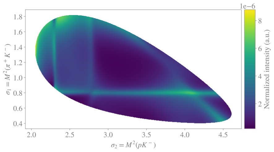
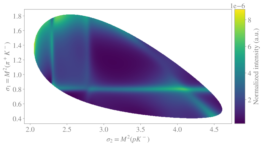
Render the Dalitz plot
fig, ax = plt.subplots(figsize=(10, 8))
mesh = ax.pcolormesh(x, y, normalized_intensities, rasterized=True)
ax.set_aspect("equal")
ax.set_xlabel(sigma_labels[i])
ax.set_ylabel(sigma_labels[j])
divider = make_axes_locatable(ax)
colorbar_axes = divider.append_axes("right", size="5%", pad=0.1)
colorbar = fig.colorbar(mesh, cax=colorbar_axes)
colorbar.ax.set_ylabel("Normalized intensity (a.u.)")
plt.show()

Render the mass projection
resonance_names = sorted({chain["name"].split("[")[0] for chain in chain_defs})


def project(intensity_values, subsystem: int):
    if subsystem == i:
        mass_values = jnp.sqrt(x[0])
        projection = jnp.nansum(intensity_values, axis=0)
    else:
        mass_values = jnp.sqrt(y[:, 0])
        projection = jnp.nansum(intensity_values, axis=1)
    return mass_values, mass_values * projection


projections = {}
normalizations = {}
for subsystem in (i, j):
    mass_values, total_projection = project(intensities, subsystem)
    projections[subsystem] = (mass_values, total_projection)
    normalizations[subsystem] = jnp.trapezoid(total_projection, mass_values)

fig, axes = plt.subplots(1, 2, figsize=(14, 6), sharey=True)
for axis, subsystem in zip(axes, (i, j), strict=True):
    mass_values, total_projection = projections[subsystem]
    axis.plot(
        mass_values,
        total_projection / normalizations[subsystem],
        color="#808080",
        lw=3,
        label="Total",
    )
for resonance_name in resonance_names:
    resonance_latex = to_latex(resonance_name)
    coupling_overrides = {
        symbol: value if resonance_latex in str(symbol) else 0
        for symbol, value in model.parameter_defaults.items()
        if str(symbol).startswith("c^")
    }
    component_workspace = compile_workspace(
        workspace,
        backend="jax",
        targets=[intensity_name],
        parameter_overrides=coupling_overrides,
    )
    component = component_workspace.functions[intensity_name](dalitz_data)
    component = jnp.where(jnp.isnan(intensities), jnp.nan, component)
    for axis, subsystem in zip(axes, (i, j), strict=True):
        mass_values, component_projection = project(component, subsystem)
        axis.plot(
            mass_values,
            component_projection / normalizations[subsystem],
            label=resonance_name,
        )
axes[0].set_xlabel(R"$m_{13}$ [GeV]")
axes[1].set_xlabel(R"$m_{23}$ [GeV]")
axes[0].set_ylabel("Normalized intensity (a.u.)")
axes[0].set_ylim(bottom=0)
handles, labels = axes[0].get_legend_handles_labels()
fig.legend(
    handles,
    labels,
    bbox_to_anchor=(0.5, 0.97),
    fontsize="small",
    loc="upper center",
    ncol=7,
)
fig.subplots_adjust(top=0.8, wspace=0.05)
plt.show()