Working with ASCII momentum tuple files

Working with ASCII momentum tuple files#

Pawian usually imports its data from momentum tuples written to an ASCII text file. Each line consists of four values: the energy and the \(x\), \(y\), \(z\)-components of the 3-momentum. The lines are grouped by event and can be preceded by an event weight. An example of two weighted events of three particles each would be:

0.99407
-0.00357645   0.0962561   0.0181079    0.170545
   0.224019    0.623156    0.215051     1.99057
  -0.174404   -0.719412   -0.233159      2.0243
0.990748
 -0.0328198   0.0524406   0.0310079    0.155783
  -0.619592    0.141315     0.32135     1.99619
   0.698477   -0.193756   -0.352357     2.03593

The pawian.data module imports such an ASCII file to a nicely formatted pandas.DataFrame and provides a few accessors that facilitate visualization of the content of the ASCII file.

The fact that we works with a pandas.DataFrame also allows one to make selections of the content and write the filtered data set to another ASCII file for Pawian (and whatever other format is already supported by pandas.DataFrame).

Import data#

In this example, we use the test files provided the pawian.data module folder in the repository.

from os.path import dirname, realpath

import pawian

sample_dir = f"{dirname(realpath(pawian.__file__))}/samples"
filename_data = f"{sample_dir}/momentum_tuples_data.dat"
filename_mc = f"{sample_dir}/momentum_tuples_mc.dat"

The data file describes momentum tuples for a \(e^+e^- \to \pi+D^0D^+\) decay (in that order!). This information can be passed on to the read_ascii() function to create a pandas.DataFrame.

from pawian.data import read_ascii

particles = ["pi+", "D0", "D-"]
frame = read_ascii(filename_data, particles=particles)
frame

Particle	pi+				D0				D-				weight
Momentum	p_x	p_y	p_z	E	p_x	p_y	p_z	E	p_x	p_y	p_z	E
0	-0.003576	0.096256	0.018108	0.170545	0.224019	0.623156	0.215051	1.99057	-0.174404	-0.719412	-0.233159	2.02430	0.994070
1	-0.032820	0.052441	0.031008	0.155783	-0.619592	0.141315	0.321350	1.99619	0.698477	-0.193756	-0.352357	2.03593	0.990748
2	0.109609	-0.192790	0.045853	0.266016	-0.303136	-0.204413	-0.444309	1.95159	0.239557	0.397203	0.398456	1.96707	0.281660
3	0.050984	-0.039164	-0.041701	0.159223	0.627018	-0.352803	-0.081468	2.00047	-0.632071	0.391967	0.123168	2.01588	0.992387
4	0.064191	0.002905	-0.062571	0.165903	0.079182	0.241238	-0.666256	1.99649	-0.097326	-0.244142	0.728827	2.02379	0.534049
...	...	...	...	...	...	...	...	...	...	...	...	...	...
995	0.208905	0.228950	0.060918	0.345326	0.011720	-0.024639	-0.443599	1.91707	-0.174541	-0.204311	0.382681	1.92720	0.179032
996	0.049370	-0.053923	0.084898	0.178976	0.363975	-0.294093	-0.565002	2.00395	-0.367383	0.348016	0.480105	1.99550	0.652028
997	0.014450	-0.050924	-0.038706	0.154208	0.420817	-0.151503	-0.588410	2.00596	-0.389284	0.202427	0.627117	2.02021	0.997076
998	-0.109077	-0.041651	0.033446	0.185016	-0.494181	-0.402043	0.058469	1.97152	0.649313	0.443694	-0.091916	2.03036	0.166129
999	-0.048741	-0.034371	0.017186	0.152749	-0.282073	-0.191036	0.642406	2.00159	0.376848	0.225407	-0.659593	2.03060	0.986252

1000 rows × 13 columns

Investigate content of the data frame#

Notice that the data frame makes use of multi-indexing for the columns. This allows us for instance to make easy selections per particle, like this:

frame["pi+"] + frame["D-"]

Momentum	p_x	p_y	p_z	E
0	-0.177980	-0.623156	-0.215051	2.194845
1	0.665657	-0.141315	-0.321349	2.191713
2	0.349166	0.204413	0.444309	2.233086
3	-0.581087	0.352803	0.081467	2.175103
4	-0.033134	-0.241237	0.666256	2.189693
...	...	...	...	...
995	0.034364	0.024639	0.443599	2.272526
996	-0.318013	0.294093	0.565003	2.174476
997	-0.374834	0.151503	0.588411	2.174418
998	0.540236	0.402043	-0.058469	2.215376
999	0.328107	0.191036	-0.642407	2.183349

1000 rows × 4 columns

frame[["pi+", "D0"]].mean()

Particle  Momentum
pi+       p_x         0.001480
          p_y         0.006563
          p_z        -0.001542
          E           0.207283
D0        p_x         0.035191
          p_y         0.000136
          p_z        -0.008241
          E           1.977187
dtype: float64

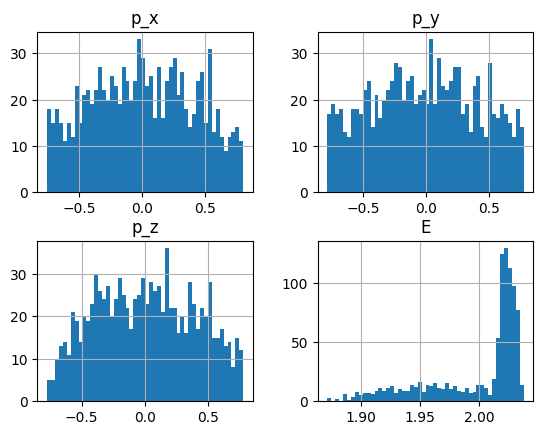
Even better, we immediately have all powerful techniques of a DataFrame at our disposal:

frame["D-"].hist(bins=50);

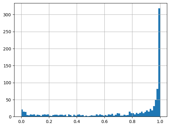
../_images/c249d187379cf5794ec8f9e0a46fa6440565dc057bdc0c02fd00c5153f762f3b.png

frame["weight"].hist(bins=80);

../_images/76d3e56a61538ce65fe51ec8420d918d0a0cd4303a03342e55a0a095c5f63bc0.png

Special accessors#

Now that we have imported from the pawian.data sub-module, a few simple accessors to the data frame have become available in the namespace pwa of the DataFrame (see PwaAccessor). They can be called from the pwa namespace like so:

print("Has weights:       ", frame.pwa.has_weights)
print("Contains particles:", frame.pwa.particles)
print("Contains momenta:  ", frame.pwa.momentum_labels)

Has weights:        True
Contains particles: ['pi+', 'D0', 'D-']
Contains momenta:   ['p_x', 'p_y', 'p_z', 'E']

The accessors also allow to get kinematic variables:

frame.pwa.p_xyz

Particle	pi+			D0			D-
Momentum	p_x	p_y	p_z	p_x	p_y	p_z	p_x	p_y	p_z
0	-0.003576	0.096256	0.018108	0.224019	0.623156	0.215051	-0.174404	-0.719412	-0.233159
1	-0.032820	0.052441	0.031008	-0.619592	0.141315	0.321350	0.698477	-0.193756	-0.352357
2	0.109609	-0.192790	0.045853	-0.303136	-0.204413	-0.444309	0.239557	0.397203	0.398456
3	0.050984	-0.039164	-0.041701	0.627018	-0.352803	-0.081468	-0.632071	0.391967	0.123168
4	0.064191	0.002905	-0.062571	0.079182	0.241238	-0.666256	-0.097326	-0.244142	0.728827
...	...	...	...	...	...	...	...	...	...
995	0.208905	0.228950	0.060918	0.011720	-0.024639	-0.443599	-0.174541	-0.204311	0.382681
996	0.049370	-0.053923	0.084898	0.363975	-0.294093	-0.565002	-0.367383	0.348016	0.480105
997	0.014450	-0.050924	-0.038706	0.420817	-0.151503	-0.588410	-0.389284	0.202427	0.627117
998	-0.109077	-0.041651	0.033446	-0.494181	-0.402043	0.058469	0.649313	0.443694	-0.091916
999	-0.048741	-0.034371	0.017186	-0.282073	-0.191036	0.642406	0.376848	0.225407	-0.659593

1000 rows × 9 columns

frame.pwa.mass.mean()

Particle
D-     1.86961
D0     1.86484
pi+    0.13957
dtype: float64

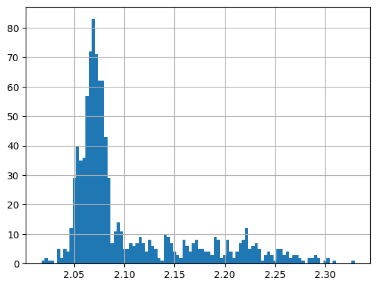
And the best part: you can just add the vectors and do analysis on for instance their combined invariant mass!

dm = frame["D-"]
pip = frame["pi+"]
(dm + pip).pwa.mass.hist(bins=100);

../_images/b6fd31b085789948e10e2c2d9d8b98c420a23c70e2a2868d802736aa31b78509.png

Selecting and exporting#

As mentioned, pandas.DataFrame allows us to make certain selections:

weights = frame["weight"]
selection = frame[weights > 0.95]
selection

Particle	pi+				D0				D-				weight
Momentum	p_x	p_y	p_z	E	p_x	p_y	p_z	E	p_x	p_y	p_z	E
0	-0.003576	0.096256	0.018108	0.170545	0.224019	0.623156	0.215051	1.99057	-0.174404	-0.719412	-0.233159	2.02430	0.994070
1	-0.032820	0.052441	0.031008	0.155783	-0.619592	0.141315	0.321350	1.99619	0.698477	-0.193756	-0.352357	2.03593	0.990748
3	0.050984	-0.039164	-0.041701	0.159223	0.627018	-0.352803	-0.081468	2.00047	-0.632071	0.391967	0.123168	2.01588	0.992387
6	-0.033936	0.042558	0.050071	0.157955	-0.591966	0.113080	0.343726	1.98972	0.671870	-0.155639	-0.393797	2.03129	0.992469
7	-0.005202	-0.042270	-0.071584	0.162536	-0.110162	-0.045471	-0.690215	1.99204	0.161362	0.087741	0.761799	2.02719	0.991051
...	...	...	...	...	...	...	...	...	...	...	...	...	...
991	-0.018286	-0.047475	-0.044260	0.155006	-0.557088	-0.343712	-0.265556	1.99415	0.621370	0.391187	0.309815	2.03238	0.991111
992	-0.001543	0.079682	-0.043369	0.166470	0.181800	0.656877	-0.171703	1.99290	-0.134226	-0.736559	0.215072	2.02540	0.998521
994	0.058329	0.050061	-0.017219	0.160265	0.354361	0.428801	-0.460858	1.99986	-0.366689	-0.478862	0.478077	2.02182	0.998338
997	0.014450	-0.050924	-0.038706	0.154208	0.420817	-0.151503	-0.588410	2.00596	-0.389284	0.202427	0.627117	2.02021	0.997076
999	-0.048741	-0.034371	0.017186	0.152749	-0.282073	-0.191036	0.642406	2.00159	0.376848	0.225407	-0.659593	2.03060	0.986252

480 rows × 13 columns

The frame can then be exported to an ASCII file that can be parsed by pawian like so:

output_file = "selected_data.dat"
selection.pwa.write_ascii(output_file)

imported_frame = read_ascii(output_file, particles)
imported_frame

Particle	pi+				D0				D-				weight
Momentum	p_x	p_y	p_z	E	p_x	p_y	p_z	E	p_x	p_y	p_z	E
0	-0.003576	0.096256	0.018108	0.170545	0.224019	0.623156	0.215051	1.99057	-0.174404	-0.719412	-0.233159	2.02430	0.994070
1	-0.032820	0.052441	0.031008	0.155783	-0.619592	0.141315	0.321350	1.99619	0.698477	-0.193756	-0.352357	2.03593	0.990748
2	0.050984	-0.039164	-0.041701	0.159223	0.627018	-0.352803	-0.081468	2.00047	-0.632071	0.391967	0.123168	2.01588	0.992387
3	-0.033936	0.042558	0.050071	0.157955	-0.591966	0.113080	0.343726	1.98972	0.671870	-0.155639	-0.393797	2.03129	0.992469
4	-0.005202	-0.042270	-0.071584	0.162536	-0.110162	-0.045471	-0.690215	1.99204	0.161362	0.087741	0.761799	2.02719	0.991051
...	...	...	...	...	...	...	...	...	...	...	...	...	...
475	-0.018286	-0.047475	-0.044260	0.155006	-0.557088	-0.343712	-0.265556	1.99415	0.621370	0.391187	0.309815	2.03238	0.991111
476	-0.001543	0.079682	-0.043369	0.166470	0.181800	0.656877	-0.171703	1.99290	-0.134226	-0.736559	0.215072	2.02540	0.998521
477	0.058329	0.050061	-0.017219	0.160265	0.354361	0.428801	-0.460858	1.99986	-0.366689	-0.478862	0.478077	2.02182	0.998338
478	0.014450	-0.050924	-0.038706	0.154208	0.420817	-0.151503	-0.588410	2.00596	-0.389284	0.202427	0.627117	2.02021	0.997076
479	-0.048741	-0.034371	0.017186	0.152749	-0.282073	-0.191036	0.642406	2.00159	0.376848	0.225407	-0.659593	2.03060	0.986252