\(\Lambda_b^0 \to p K^- \gamma\) This page demonstrates deserialization and evaluation of an amplitude model for the decay \(\Lambda_b^0 \to p K^- \gamma\) . The resonant structure was studied using proton-proton collision data recorded at centre-of-mass energies of \(7\) , \(8\) , and \(13\) TeV with the LHCb detector, INSPIRE-HEP 2765817 .
Import Python libraries
from copy import deepcopyfrom pathlib import Pathimport jsonimport loggingimport jax.numpy as jnpimport matplotlib.pyplot as pltimport pandas as pdimport sympy as spfrom ampform.dynamics.form_factor import BreakupMomentumSquaredfrom ampform_dpd import DefinedExpressionfrom ampform_dpd.decay import FinalStateID, State, ThreeBodyDecayfrom ampform_dpd.io import aslatex, cached, perform_cached_lambdifyfrom ampform_dpd.io.serialization import amplitude as serialization_amplitudefrom ampform_dpd.io.serialization.amplitude import formulatefrom ampform_dpd.io.serialization.decay import get_final_state, to_decayfrom ampform_dpd.io.serialization.dynamics import (from ampform_dpd.io.serialization.format import (from IPython.display import Mathfrom matplotlib_inline.backend_inline import set_matplotlib_formatsfrom mpl_toolkits.axes_grid1 import make_axes_locatable # cspell:ignore mpl_toolkits = Path("." ).absolute()"ampform.sympy" ).setLevel(logging.ERROR)"svg" )
with open (THIS_DIR.parent.parent / "models" / "lb2pkg-lhcb-2765817.json" ) as f:= json.load(f)
Name-to-LaTeX converter
def to_latex(name: str ) -> str := {"Lb" : R"\Lambda_b^0" ,"g" : R"\gamma" ,"K" : "K^-" ,"p" : "p" ,if latex is not None :return latexif name.startswith("LNR" ):return R"\Lambda_\mathrm {NR} " if name.startswith("L" ):return Rf"\Lambda( { name[1 :]} )" return name= to_decay(MODEL_DEFINITION, to_latex= to_latex)= True ))
\(\displaystyle \begin{array}{c}
\Lambda_b^0\left[J=\frac{1}{2}\right] \to \left(\Lambda(1405)\left[J=\frac{1}{2}\right] \to p\left[J=\frac{1}{2}\right] K^-\left[J=0\right]\right) \gamma\left[J=1\right] \\
\Lambda_b^0\left[J=\frac{1}{2}\right] \to \left(\Lambda(1520)\left[J=\frac{3}{2}\right] \to p\left[J=\frac{1}{2}\right] K^-\left[J=0\right]\right) \gamma\left[J=1\right] \\
\Lambda_b^0\left[J=\frac{1}{2}\right] \to \left(\Lambda(1600)\left[J=\frac{1}{2}\right] \to p\left[J=\frac{1}{2}\right] K^-\left[J=0\right]\right) \gamma\left[J=1\right] \\
\Lambda_b^0\left[J=\frac{1}{2}\right] \to \left(\Lambda(1670)\left[J=\frac{1}{2}\right] \to p\left[J=\frac{1}{2}\right] K^-\left[J=0\right]\right) \gamma\left[J=1\right] \\
\Lambda_b^0\left[J=\frac{1}{2}\right] \to \left(\Lambda(1690)\left[J=\frac{3}{2}\right] \to p\left[J=\frac{1}{2}\right] K^-\left[J=0\right]\right) \gamma\left[J=1\right] \\
\Lambda_b^0\left[J=\frac{1}{2}\right] \to \left(\Lambda(1800)\left[J=\frac{1}{2}\right] \to p\left[J=\frac{1}{2}\right] K^-\left[J=0\right]\right) \gamma\left[J=1\right] \\
\Lambda_b^0\left[J=\frac{1}{2}\right] \to \left(\Lambda(1810)\left[J=\frac{1}{2}\right] \to p\left[J=\frac{1}{2}\right] K^-\left[J=0\right]\right) \gamma\left[J=1\right] \\
\Lambda_b^0\left[J=\frac{1}{2}\right] \to \left(\Lambda(1820)\left[J=\frac{5}{2}\right] \to p\left[J=\frac{1}{2}\right] K^-\left[J=0\right]\right) \gamma\left[J=1\right] \\
\Lambda_b^0\left[J=\frac{1}{2}\right] \to \left(\Lambda(1830)\left[J=\frac{5}{2}\right] \to p\left[J=\frac{1}{2}\right] K^-\left[J=0\right]\right) \gamma\left[J=1\right] \\
\Lambda_b^0\left[J=\frac{1}{2}\right] \to \left(\Lambda(1890)\left[J=\frac{3}{2}\right] \to p\left[J=\frac{1}{2}\right] K^-\left[J=0\right]\right) \gamma\left[J=1\right] \\
\Lambda_b^0\left[J=\frac{1}{2}\right] \to \left(\Lambda(2100)\left[J=\frac{7}{2}\right] \to p\left[J=\frac{1}{2}\right] K^-\left[J=0\right]\right) \gamma\left[J=1\right] \\
\Lambda_b^0\left[J=\frac{1}{2}\right] \to \left(\Lambda(2110)\left[J=\frac{5}{2}\right] \to p\left[J=\frac{1}{2}\right] K^-\left[J=0\right]\right) \gamma\left[J=1\right] \\
\Lambda_b^0\left[J=\frac{1}{2}\right] \to \left(\Lambda(2350)\left[J=\frac{9}{2}\right] \to p\left[J=\frac{1}{2}\right] K^-\left[J=0\right]\right) \gamma\left[J=1\right] \\
\Lambda_b^0\left[J=\frac{1}{2}\right] \to \left(\Lambda_\mathrm{NR}\left[J=\frac{3}{2}\right] \to p\left[J=\frac{1}{2}\right] K^-\left[J=0\right]\right) \gamma\left[J=1\right] \\
\end{array}\)
Dynamics
The model contains Breit-Wigner and multichannel Breit-Wigner propagators, as well as a constant non-resonant term. The latter is serialized as a zeroth-order polynomial.
= get_decay_chains(MODEL_DEFINITION)= {"parametrization" ]: chainfor chain in CHAIN_DEFSfor propagator in chain["propagators" ]
= formulate_dynamics(chains_by_propagator["L1520_BW" ], MODEL_DEFINITION)
\(\displaystyle \begin{array}{rcl}
\mathcal{R}^\mathrm{BW}_{L=2}\left(\sigma_{3}; m_{L1520}, \Gamma_{L1520}\right) &=& \mathcal{R}^\mathrm{BW}\left(\sigma_{3}; m_{L1520}, \Gamma_{1520}\left(\sigma_{3}\right)\right) \\
m_{L1520} &=& 1.519 \\
\Gamma_{L1520} &=& 0.016 \\
m_{1} &=& 0.938 \\
m_{2} &=& 0.493 \\
R_\mathrm{res} &=& 1.5 \\
\end{array}\)
= formulate_dynamics("L1405_Flatte" ],
\(\displaystyle \begin{array}{rcl}
\mathcal{R}^\mathrm{BW}_\mathrm{multi}\left(\sigma_{3}; \Gamma_{L1405}, \Gamma_{L1405}^\text{ch. 2}\right) &=& \mathcal{R}^\mathrm{BW}_{L=0}\left(\sigma_{3}; m_{L1405}, \Gamma^\text{ch}\left(\sigma_{3}; m_{L1405}, \Gamma_{L1405}\right) + \Gamma^\text{ch}\left(\sigma_{3}; m_{L1405}, \Gamma_{L1405}^\text{ch. 2}\right)\right) \\
m_{L1405} &=& 1.405 \\
\Gamma_{L1405} &=& 0.24941478752959237 \\
m_{1} &=& 0.938 \\
m_{2} &=& 0.493 \\
R_{L1405} &=& 0 \\
m_{a,2} &=& 1.197 \\
m_{b,2} &=& 0.14 \\
\Gamma_{L1405}^\text{ch. 2} &=& 0.24941478752959237 \\
\end{array}\)
Construct amplitude model
The current Python preview API needs two small compatibility adapters for this older LS-coupled model. They preserve a unique symbol for every serialized LS coupling and implement the serialized MomentumPower and constant Polynomial functions.
Compatibility adapters for LS-coupled models
def prepare_ls_model(model_definition: dict ) -> dict := deepcopy(model_definition)= get_decay_chains(model_definition)for chain_idx, chain in enumerate (chains):for vertex in chain["vertices" ]:if "helicities" in vertex:continue = any (isinstance (item, list ) for item in vertex["node" ])"helicities" ] = [str (chain_idx), "0" ] if has_isobar else ["0" , "0" ]return model_definitiondef get_ls_child_spins(model_definition, chain_idx, vertex_idx):= get_decay_chains(model_definition)[chain_idx]= chain["vertices" ][vertex_idx]= get_final_state(model_definition)= sp.Rational(chain["propagators" ][0 ]["spin" ])return tuple (if isinstance (item, int ) else resonance_spinfor item in vertex["node" ]def formulate_polynomial(propagator, resonance, model):= get_function_definition(propagator["parametrization" ], model)= to_mandelstam_symbol(propagator["node" ])= sum (* variable** powerfor power, coefficient in enumerate (definition["coefficients" ])return DefinedExpression(expression= expression)= serialization_amplitude.formulate_form_factordef formulate_form_factor(vertex, model):= vertex.get("formfactor" )if not function_name:return DefinedExpression()= get_function_definition(function_name, model)if definition["type" ] != "MomentumPower" :return _original_formulate_form_factor(vertex, model)= vertex["node" ]if all (isinstance (item, int ) for item in node):= to_mandelstam_symbol(node)= (to_mass_symbol(item) for item in node)else := to_mandelstam_symbol(node) ** 2 = (to_mass_symbol(item) for item in node)= sp.sqrt(m1)= sp.Rational(definition["l" ], 2 )return DefinedExpression(expression= BreakupMomentumSquared(s, m1, m2) ** power)= get_ls_child_spins= formulate_form_factor= prepare_ls_model(MODEL_DEFINITION)= {"Polynomial" : formulate_polynomial}
= formulate(= True ,= to_latex,= ADDITIONAL_BUILDERS,
Validation
The table compares all serialized checkpoints with the Python implementation. The marks “🟢”, “🟡”, and “🔴” indicate an absolute difference of \(<10^{-10}\) , \(<10^{-2}\) , or \(\ge10^{-2}\) , respectively.
Validation helpers
= {"name" ]: {parameter["name" ]: parameter["value" ] for parameter in point["parameters" ]}for point in MODEL_DEFINITION["parameter_points" ]def to_number(value: float | str ) -> float | complex :if isinstance (value, str ):= complex (value.replace(" " , "" ).replace("i" , "j" ))= complex (value)return number.real if number.imag == 0 else numberdef round_number(value: float | complex , digits: int = 6 ) -> float | complex := complex (value)if number.imag == 0 :return round (number.real, digits)return complex (round (number.real, digits), round (number.imag, digits))def label_diff(difference: complex ) -> str := abs (difference)if absolute_difference < 1e-10 :return "🟢" if absolute_difference < 1e-2 :return "🟡" return "🔴" def create_intensity_function(int ,str | None = None ,= next (s for s in model.invariants if str (s) == f"sigma { subsystem} " )= cached.xreplace(cached.unfold(model), model.variables)= select_resonance_parameters(model, resonance_name)= cached.xreplace(intensity_expr, parameter_defaults)= model.invariants[invariant].xreplace(model.masses).doit()= cached.doit(intensity_expr.xreplace({invariant: invariant_expr}))return cached.lambdify(intensity_expr, backend= "jax" )def select_resonance_parameters(model, resonance_name: str | None ):if resonance_name is None :return model.parameter_defaultsreturn {if not str (symbol).startswith("c^" ) or resonance_name in str (symbol)else 0 for symbol, value in model.parameter_defaults.items()def evaluate_intensity(model, point: dict [str , float ], pair: tuple [int , int ]) -> float := pair* _ = {1 , 2 , 3 } - set (pair)= {str (s): s for s in model.invariants}= invariants[f"sigma { j} " ]= invariants[f"sigma { k} " ]= next (for angle, expression in model.variables.items()if str (angle) == f"theta_ { i}{ j} " = point[f"m_ { i}{ j} " ] ** 2 = sp.Eq(f"cos_theta_ { i}{ j} " ],= sp.solve(equation.subs(sigma_k, sigma_k_value), sigma_j)[0 ]= create_intensity_function(model, subsystem= i)= function({str (sigma_j): float (sigma_j_value), str (sigma_k): sigma_k_value})return float (jnp.real(value))
Compute every serialized checkpoint
= []for checksum in MODEL_DEFINITION["misc" ]["amplitude_model_checksums" ]:= checksum["distribution" ]= checksum_points[checksum["point" ]]= to_number(checksum["value" ])= chains_by_propagator.get(distribution_name)if chain is None := evaluate_intensity(model, point, pair= (1 , 2 ))else := formulate_dynamics(= ADDITIONAL_BUILDERS,= dynamics.expression.doit()= expression.free_symbols - dynamics.parameters.keys()if variables:= perform_cached_lambdify(= dynamics.parameters,= next (iter (variables))= function({str (variable): next (iter (point.values()))})else := complex (expression.xreplace(dynamics.parameters))= abs (reference_value - computed_value)"Distribution" : distribution_name,"Point" : checksum["point" ],"Reference" : round_number(reference_value),"Computed" : round_number(computed_value),"Difference" : difference,"Status" : label_diff(reference_value - computed_value),= object )
0
default_model
validation_point1
645.687778
644.103426
1.584352
🔴
1
default_model
validation_point2
33.313132
33.314165
0.001032
🟡
2
default_model
validation_point3
38.286729
38.287889
0.00116
🟡
3
L1405_Flatte
validation_point_m12sq
(-0.740198+0.236368j)
(-0.775611+0.176283j)
0.06974548265443277
🔴
4
L1890_BW
validation_point_m12sq
(2.198693+1.036641j)
(2.198693+1.036641j)
0.0
🟢
5
L1800_BW
validation_point_m12sq
(0.311734+2.7742j)
(0.311734+2.7742j)
4.577566798522237e-16
🟢
6
L1520_BW
validation_point_m12sq
(-0.643171+0.553948j)
(-0.643171+0.553948j)
2.482534153247273e-16
🟢
7
L2110_BW
validation_point_m12sq
(0.854068+0.041564j)
(0.854068+0.041564j)
1.2738115944464653e-16
🟢
8
L1680_BW
validation_point_m12sq
(-2.46133+0.361098j)
(-2.46133+0.361098j)
1.1102230246251565e-16
🟢
9
L2350_BW
validation_point_m12sq
(0.43057+0.000197j)
(0.43057+0.000197j)
1.0028870095490916e-18
🟢
10
L1600_BW
validation_point_m12sq
(-0.629331+0.766337j)
(-0.629331+0.766337j)
2.220446049250313e-16
🟢
11
L1810_BW
validation_point_m12sq
(0.106436+5.093986j)
(0.106436+5.093986j)
8.899114524108741e-16
🟢
12
L1820_BW
validation_point_m12sq
(4.647408+4.443945j)
(4.647408+4.443945j)
4.440892098500626e-15
🟢
13
L1830_BW
validation_point_m12sq
(3.824528+3.82775j)
(3.824528+3.82775j)
1.7763568394002505e-15
🟢
14
L2100_BW
validation_point_m12sq
(0.826225+0.013532j)
(0.826225+0.013532j)
1.5612511283791264e-17
🟢
15
L1690_BW
validation_point_m12sq
(-1.859729+1.396126j)
(-1.859729+1.396126j)
1.4043333874306805e-15
🟢
16
LNR30_NR
validation_point_m12sq
1.0
1.0
0.0
🟢
Visualization
Dalitz plot
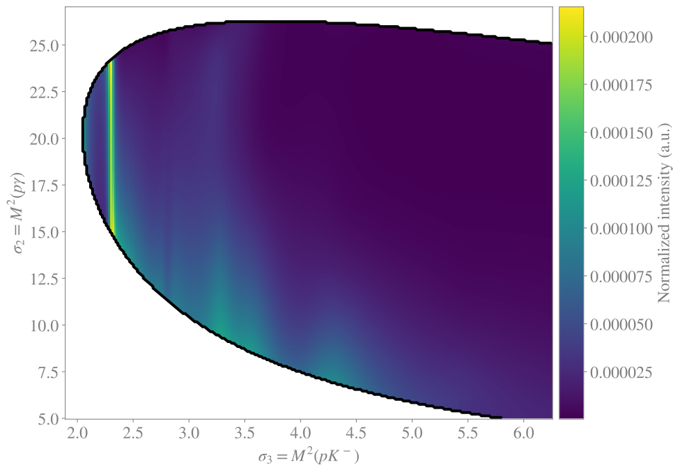
The Dalitz plot shows the intensity up to \(m_{pK^-}=2.5\ \mathrm{GeV}\) . The plotting range includes a margin below the physical threshold so that the left phase-space boundary remains visible, as in the Julia implementation.
Configure the Dalitz plot
= 3 , 2 * _ = {1 , 2 , 3 } - {x_subsystem, y_subsystem}= 250 = 1.9 , 2.5 ** 2 = 5 , 27 = jnp.meshgrid(= create_intensity_function(model, subsystem= eliminated_subsystem)= jnp.real(intensity_function({f"sigma { x_subsystem} " : X,f"sigma { y_subsystem} " : Y,= intensities / jnp.nansum(intensities)def get_decay_products(-> tuple [State, State]:return tuple (state for state in decay.final_state.values() if state.index != subsystem)= {Rf"$\sigma_ { subsystem} = M^2\left( { ' ' . join(p.latex for p in get_decay_products(DECAY, subsystem))} \right)$" for subsystem in (1 , 2 , 3 )# cspell:ignore bbox edgecolor facecolor fontset fontsize labelcolor mathtext ncol # cspell:ignore savefig sharey startswith STIX wspace xtick ytick "axes.edgecolor" : "#808080" ,"axes.facecolor" : "none" ,"axes.labelcolor" : "#808080" ,"figure.facecolor" : "none" ,"font.family" : "serif" ,"font.serif" : ["STIXGeneral" , "DejaVu Serif" ],"font.size" : 18 ,"mathtext.fontset" : "stix" ,"savefig.transparent" : True ,"text.color" : "#808080" ,"xtick.color" : "#808080" ,"ytick.color" : "#808080" ,
Render the Dalitz plot
= plt.subplots(figsize= (10 , 8 ))= ax.pcolormesh(X, Y, normalized_intensities, rasterized= True )= [0.5 ],= "black" ,= 3 ,= make_axes_locatable(ax)= divider.append_axes("right" , size= "5%" , pad= 0.1 )= fig.colorbar(mesh, cax= colorbar_axes)"Normalized intensity (a.u.)" )
Mass projection
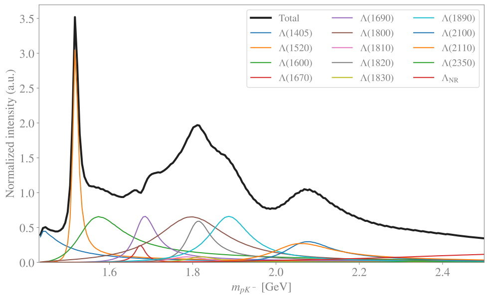
The projection onto the \(pK^-\) mass is shown as a black line. The colored curves show the incoherent contribution from each \(\Lambda\) resonance.
Render the proton-kaon mass projection
= sorted ({chain["name" ] for chain in CHAIN_DEFS})= jnp.sqrt(X[0 ])= float ("m1" , nonnegative= True ) + sp.Symbol("m2" , nonnegative= True )= mass_values >= minimum_mass= mass_values[physical_region]def project_to_pk(intensity_values):= jnp.nansum(intensity_values, axis= 0 )return mass_values * projection[physical_region]= project_to_pk(intensities)= jnp.trapezoid(total_projection, mass_values)= plt.subplots(figsize= (12 , 7 ))/ normalization,= "#202020" ,= 3 ,= "Total" ,for resonance_name in resonance_names:= create_intensity_function(= eliminated_subsystem,= to_latex(resonance_name),= jnp.real(component_function({"sigma2" : Y, "sigma3" : X}))= jnp.where(jnp.isnan(intensities), jnp.nan, component)= Rf"$ { to_latex(resonance_name)} $" / normalization,= label,R"$m_{pK^-}$ [GeV]" )"Normalized intensity (a.u.)" )2.5 )= 0 )= "small" , loc= "upper right" , ncol= 3 )