Transformers

How language models work

Mikhail Mikhasenko · Lecture 4A

Generative models

A classifier learns p(y∣x)p(y\mid x): which label for this input?

A generative model learns the distribution of the data itself, p(x)p(x), and can sample new examples from it.

With a condition, it samples p(x∣prompt)p(x\mid\text{prompt}):

  • an image given a description
  • a text given the start of a text

Language models are generative models of text.

Generated painting of a crocodile drinking tea in an armchair, watching a turtle through the window

“A painted picture of a crocodile in the house drinking tea and waiting for a turtle to visit”

A language model predicts the next token

Split text into tokens x1,…,xTx_1,\dots,x_T. By the chain rule of probability,

p(x1,…,xT)=∏t=1Tp(xt∣x1,…,xt−1).p(x_1,\dots,x_T)=\prod_{t=1}^{T}p\left(x_t\mid x_1,\dots,x_{t-1}\right).

So one task is enough: given the text so far, give a probability for every possible next token.

Generate by sampling a token, appending it, and repeating.

GPT-2 (124 M parameters, 2019):

text so far next token
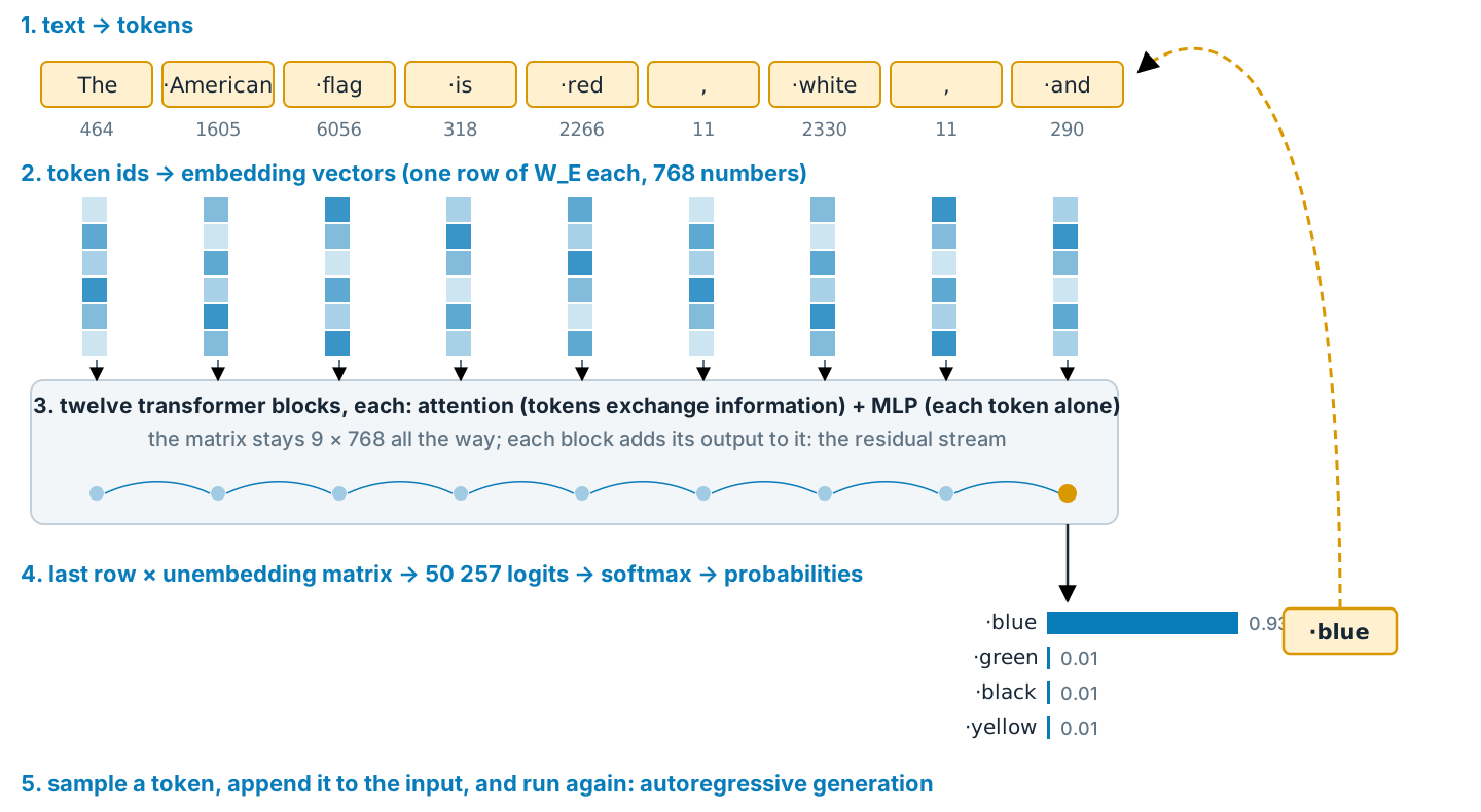
The American flag is red, white, and blue 0.93
When Mary and John went to the store, John gave a drink to Mary 0.68
The capital of France is the 0.08, now 0.05, … Paris 0.03

Llama 3.2 (1.2 B, 2024) gives Paris 0.39.

The whole machine on one slide

Text is split into tokens, tokens become embedding vectors, twelve transformer blocks update them, the last vector is turned into probabilities over the vocabulary, and the sampled token is appended to the input

Why tokens?

Unit Vocabulary Length of a text Problem
characters ~100 (bytes: 256) long: one step per letter the model must learn spelling before meaning
words millions short new words, typos, names and other languages are unknown
subword tokens 50 k – 200 k ~4 characters per token in English a compromise, learned from data

Frequent words become single tokens (·the, ·electron); rare words are split into pieces (·Bo ch um).

Byte-pair encoding

Training the tokenizer
  1. Start with single symbols (GPT-2: the 256 possible bytes).
  2. Count all adjacent pairs in a large text.
  3. Merge the most frequent pair into a new symbol.
  4. Repeat until the vocabulary has the desired size.

GPT-2: 256 bytes + 50 000 merges + 1 end-of-text token = 50 257.

Using it

Split new text into bytes, then apply the learned merges in the order they were learned.

Starting from bytes, nothing is ever “unknown”: any text, any language, any emoji can be encoded.

The tokenizer is trained once, before the network, and is not changed by gradient descent.

Byte-pair encoding, merge by merge

Real tokenizers

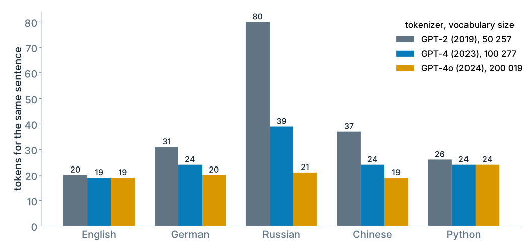
Number of tokens for the same sentence in English, German, Russian, Chinese and Python for three OpenAI tokenizers

text GPT-2 tokens
strawberry st raw berry
·Bochum ·Bo ch um
·Energieerhaltungssatz 9 pieces
·12345678 ·123 45 678
·SolidGoldMagikarp 1 token

The model never sees letters: counting the r’s in strawberry is hard.

Embedding: a token becomes a vector

Each token id ii selects one row of the embedding matrix WEW_E:

𝐞i=WE⊤𝟏i∈ℝd,WE∈ℝV×d.\mathbf e_i=W_E^{\top}\,\mathbf 1_i\in\mathbb R^{d},\qquad W_E\in\mathbb R^{V\times d}.

A one-hot vector times a matrix: a lookup table, trained by backpropagation like any other weight.

GPT-2: V=50257V=50\,257, d=768d=768, so WEW_E has 38.6 M of the 124 M parameters.

Training moves tokens that are used in similar contexts to similar vectors:

  • nearest to Monday: Tuesday, Thursday, Wednesday, Friday
  • nearest to electron: electrons, photon, neutron
  • king − man + woman ≈ queen
  • Paris − France + Germany ≈ Berlin

The same idea as AlexNet’s fc7 embedding in Lecture 3B.

Token embeddings of GPT-2

Where is each token?

Attention (next slides) compares tokens by content only. Shuffle the input and each token gets the same result: “dog bites man” = “man bites dog”.

So add information about the position t=1,2,…t=1,2,\dots to each token vector:

𝐱t=𝐞token(t)+𝐩t∈ℝd\mathbf x_t=\mathbf e_{\text{token}(t)}+\mathbf p_t\ \in\mathbb R^{d}

  • 𝐞token(t)\mathbf e_{\text{token}(t)}: embedding of the token at position tt (a row of WEW_E)
  • 𝐩t\mathbf p_t: position vector, same size dd
  • mm: index of a coordinate pair, m=0,…,d/2−1m=0,\dots,d/2-1
model position encoding
Transformer (2017) fixed: pt,2m=sinωmt,pt,2m+1=cosωmtp_{t,2m}=\sin\omega_m t,\ p_{t,2m+1}=\cos\omega_m t
GPT-2 (2019) learned 𝐩t\mathbf p_t per position, up to 1024
Llama, most since 2023 RoPE (rotary), below

RoPE. Attention compares a query 𝐪\mathbf q and a key 𝐤\mathbf k (next slides) by the dot product 𝐪⋅𝐤\mathbf q\cdot\mathbf k. Instead of adding 𝐩t\mathbf p_t, rotate each coordinate pair (q2m,q2m+1)(q_{2m},q_{2m+1}) by the angle ωmt\omega_m t:

(q2mq2m+1)→(cosωmt−sinωmtsinωmtcosωmt)(q2mq2m+1)\begin{pmatrix}q_{2m}\\q_{2m+1}\end{pmatrix}\to\begin{pmatrix}\cos\omega_m t&-\sin\omega_m t\\\sin\omega_m t&\cos\omega_m t\end{pmatrix}\begin{pmatrix}q_{2m}\\q_{2m+1}\end{pmatrix}

with ωm=10000−2m/d\omega_m=10000^{-2m/d}, and the same for 𝐤\mathbf k. Rotations keep lengths, so the score changes only through the angle ωm(t−t′)\omega_m(t-t'): it depends on the distance between the two tokens.

Why attention?

The meaning of a token depends on other tokens, sometimes far away:

  • the bank of the river / the bank raised its rates
  • The electron was accelerated in the field, and it …
  • The American flag is red, white, and …

Each position must collect information from the relevant other positions, whose number and location change from text to text.

A dense layer has one fixed weight per input position: it cannot route information by content.

Recurrent networks (before 2017) passed a single state vector along the text: slow, one step at a time, and forgetful over long distances.

Attention: every token asks a question, every token offers an answer, and the weights are computed from the data.

Query, key, value

From each token vector 𝐱i\mathbf x_i compute three vectors with learned matrices:

𝐪i=WQ𝐱i,𝐤i=WK𝐱i,𝐯i=WV𝐱i\mathbf q_i=W_Q\mathbf x_i,\qquad \mathbf k_i=W_K\mathbf x_i,\qquad \mathbf v_i=W_V\mathbf x_i

  • query: what am I looking for?
  • key: what do I contain?
  • value: what do I pass on if selected?

Similarity is the dot product 𝐪i⋅𝐤j\mathbf q_i\cdot\mathbf k_j, the same similarity score as a CNN kernel on an image patch.

The output for token ii is a weighted average of values:

𝐨i=∑jaij𝐯j,aij=e𝐪i⋅𝐤j/dk∑j′e𝐪i⋅𝐤j′/dk\mathbf o_i=\sum_j a_{ij}\,\mathbf v_j,\qquad a_{ij}=\frac{e^{\mathbf q_i\cdot\mathbf k_j/\sqrt{d_k}}}{\sum_{j'} e^{\mathbf q_i\cdot\mathbf k_{j'}/\sqrt{d_k}}}

Weights aij≥0a_{ij}\ge 0, ∑jaij=1\sum_j a_{ij}=1: a softmax over all tokens.

GPT-2: 𝐱∈ℝ768\mathbf x\in\mathbb R^{768}, 𝐪,𝐤,𝐯∈ℝ64\mathbf q,\mathbf k,\mathbf v\in\mathbb R^{64} per head.

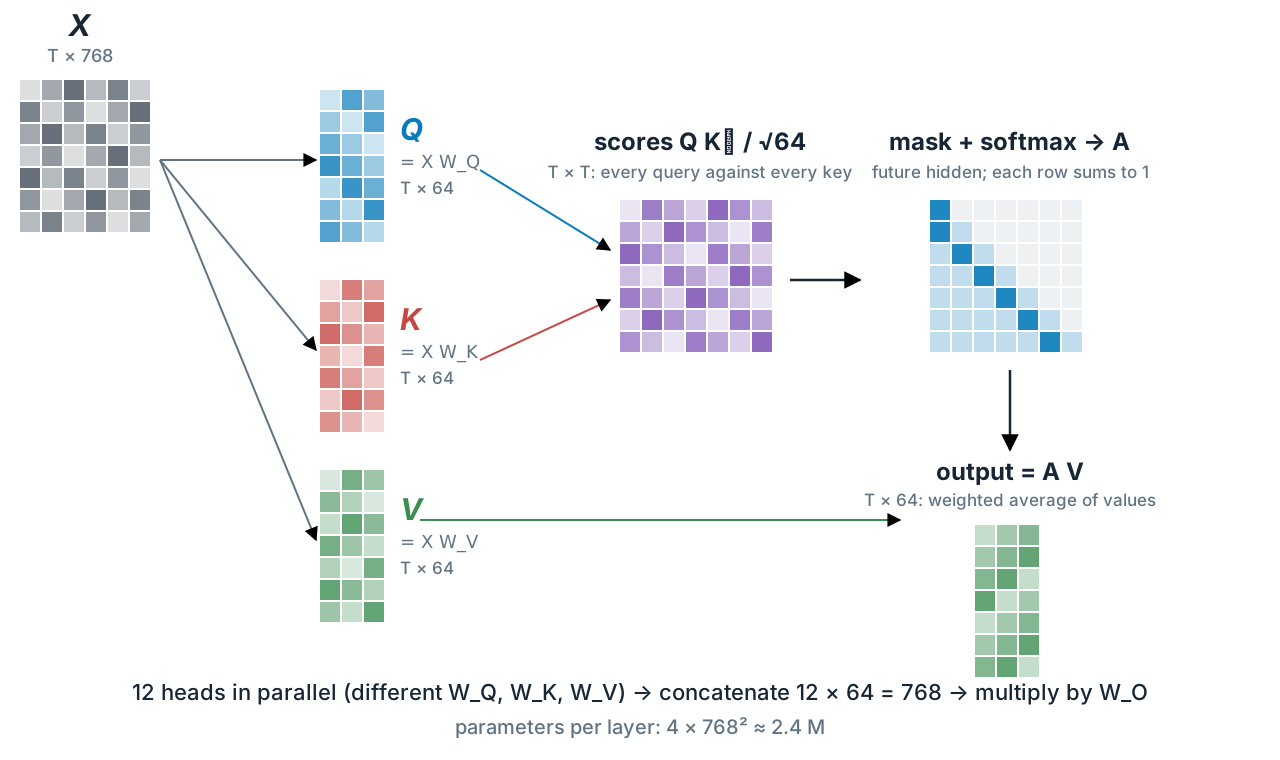
Scaled dot-product attention

The input matrix X is multiplied by three weight matrices to give Q, K and V; Q times K transposed gives a T by T score matrix, which is masked, passed through softmax, and multiplied by V

Attention(Q,K,V)=softmax(QK⊤dk+M)V,Mij={0j≤i−∞j>i\operatorname{Attention}(Q,K,V)=\operatorname{softmax}\!\left(\frac{QK^{\top}}{\sqrt{d_k}}+M\right)V,\qquad M_{ij}=\begin{cases}0 & j\le i\\ -\infty & j>i\end{cases}

Dividing by dk\sqrt{d_k}: for random vectors Var(𝐪⋅𝐤)=dk\operatorname{Var}(\mathbf q\cdot\mathbf k)=d_k, and large scores would saturate the softmax.

Attention by hand: which bank?

Multi-head attention

One attention pattern can express one kind of relation. So run hh heads in parallel, each with its own WQ(k),WK(k),WV(k)W_Q^{(k)},W_K^{(k)},W_V^{(k)} of size d×d/hd\times d/h:

MHA(X)=[𝐨(1)⋯𝐨(h)]WO\operatorname{MHA}(X)=\big[\,\mathbf o^{(1)}\,\cdots\,\mathbf o^{(h)}\,\big]\,W_O

Heads specialize: previous word, subject of the verb, matching bracket, earlier copy of the current word…

GPT-2 small GPT-3 DeepSeek-R1
layers 12 96 61
heads per layer 12 96 128
width dd 768 12 288 7 168
attention patterns 144 9 216 7 808

Parameters per attention layer: 4d24d^2 (plus biases).

What GPT-2’s heads look at

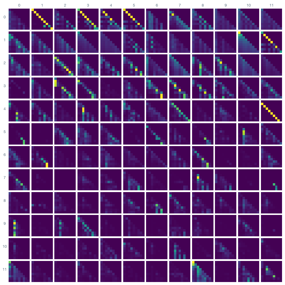
The 144 attention patterns of GPT-2 small for the text The American flag is red, white, and

All 144 attention patterns of GPT-2 for “The American flag is red, white, and” (rows: layers 0–11, columns: heads 0–11).

Some roles are known:

  • L4 H11: the previous token
  • L5 H5, L6 H9: induction heads (next slide)
  • L9 H9, L9 H6: move a name to the output (“John gave a drink to … Mary”)

Most heads have no simple description.

Inside GPT-2: 144 attention heads

Induction heads: learning inside the prompt

A two-head circuit:

  1. a previous-token head writes into each token “the word before me was A”;
  2. an induction head at the current token B searches for earlier tokens whose previous word was B, and copies what followed.

Pattern: … A B … A → predict B.

Random words shown twice: GPT-2’s loss falls from 11.8 to 0.73 nats per token.
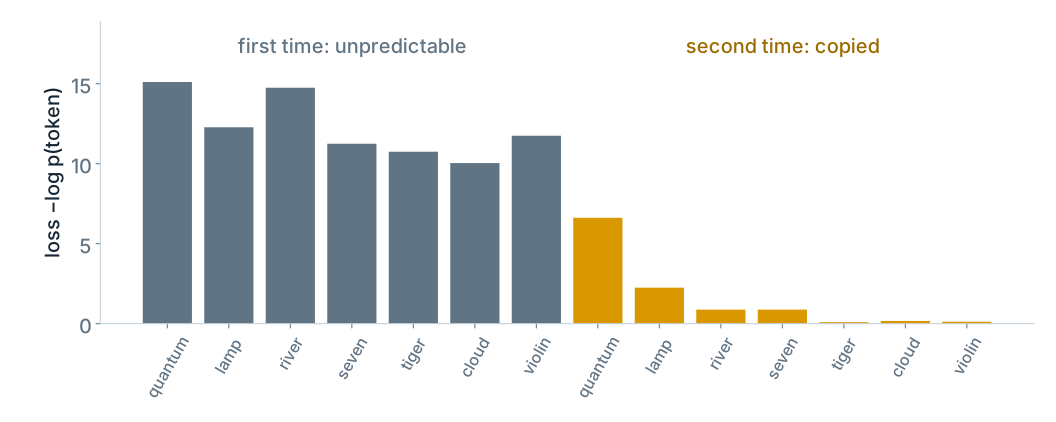
Per-token loss of GPT-2 on seven random words repeated twice: high the first time, near zero the second time

The transformer block

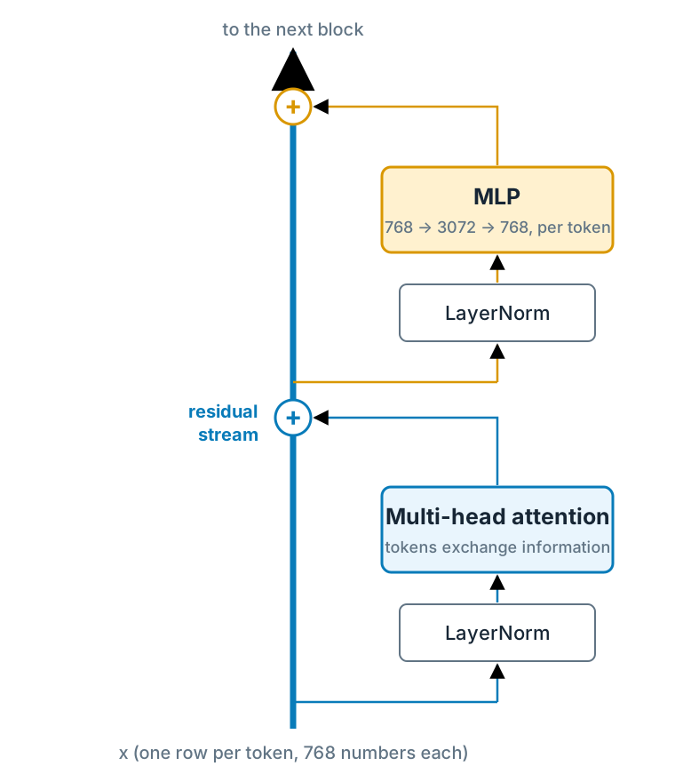
A transformer block: layer norm and multi-head attention added to the residual stream, then layer norm and an MLP added to the residual stream

Attention: tokens exchange information.

MLP: each token processed on its own, 768→3072→768768\to3072\to768 with GELU. Two thirds of the block’s weights; much of the model’s factual knowledge seems to live here.

LayerNorm (LN): rescale each token vector to mean 0 and spread 1 before it enters attention or the MLP (next slide).

Residual connections: each block adds to 𝐱\mathbf x, as in ResNet (Lecture 3B): 𝐱←𝐱+Attn(LN(𝐱)),𝐱←𝐱+MLP(LN(𝐱))\mathbf x\leftarrow\mathbf x+\operatorname{Attn}(\operatorname{LN}(\mathbf x)),\quad \mathbf x\leftarrow\mathbf x+\operatorname{MLP}(\operatorname{LN}(\mathbf x))

GPT-2 small stacks 12 blocks, GPT-3 96.

LayerNorm

Take one token vector 𝐱=(x1,…,xd)\mathbf x=(x_1,\dots,x_d), d=768d=768. Compute its mean and spread over the dd features:

μ=1d∑j=1dxj,σ=1d∑j=1d(xj−μ)2\mu=\frac1d\sum_{j=1}^{d}x_j,\qquad \sigma=\sqrt{\frac1d\sum_{j=1}^{d}(x_j-\mu)^2}

Standardize, then scale and shift each feature jj:

LN(𝐱)j=γjxj−μσ+βj\operatorname{LN}(\mathbf x)_j=\gamma_j\,\frac{x_j-\mu}{\sigma}+\beta_j

  • 𝛄,𝛃∈ℝd\boldsymbol\gamma,\boldsymbol\beta\in\mathbb R^{d}: learned, like weights and biases
  • each token alone: rows of the T×dT\times d matrix do not mix
  • batch normalization (Lecture 3A) averages one unit over the batch; LayerNorm averages one token over its features

Why? Every block adds to the residual stream, so its scale grows. GPT-2, last token of “The American flag is red, white, and”:

entering μ\mu σ\sigma largest |xj|\lvert x_j\rvert
block 1 0.00 0.17 1.2
block 2 0.01 1.96 26
block 7 −0.02 2.73 30
block 12 0.16 7.59 98

After LN: μ=0\mu=0, σ=1\sigma=1 at every depth. Attention and the MLP always see inputs of the same size; the stream itself keeps growing.

GPT-2 has 25 LayerNorms (2 per block + 1 before the unembedding): 25×2×768=3840025\times2\times768=38\,400 parameters.

The residual stream: watching a prediction form
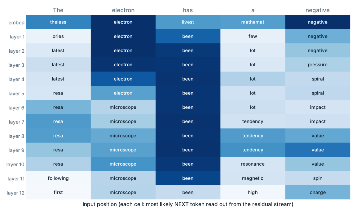
Logit lens for The electron has a negative: the most likely next token read out after each layer, with charge appearing only at the last layer

Each block adds a little to a running vector per token: the residual stream.

Logit lens: read the stream out early with the final unembedding.

After “negative”, GPT-2’s guess moves from pressure to impact, value, spin and finally charge (0.47) in the last layer.

Encoders and decoders
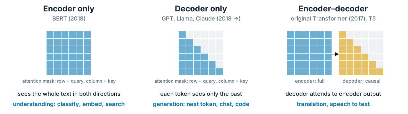
Three transformer families: encoder only with full attention, decoder only with causal attention, and encoder-decoder with cross-attention

The 2017 Transformer translated: an encoder read the German sentence, a decoder wrote the English one and looked at the encoder through cross-attention. GPT kept only the decoder, and one objective, next-token prediction, turned out to cover almost every task.

Training: predict every next token
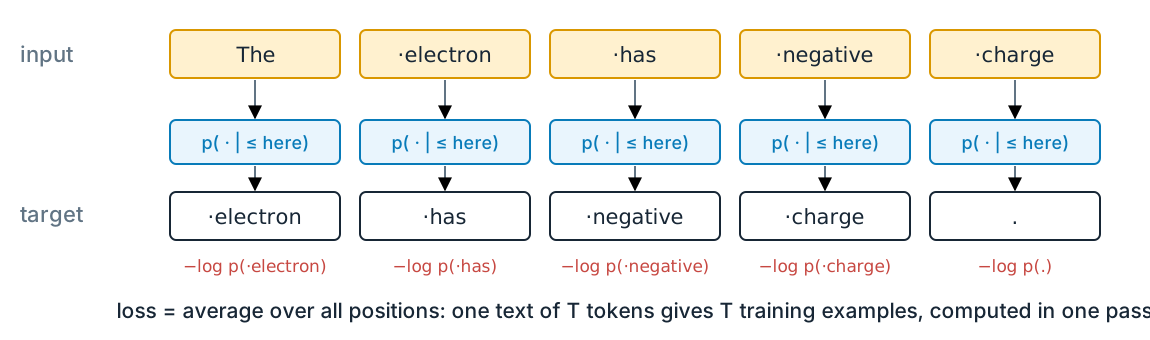
The input tokens shifted by one position are the targets; each position contributes a cross-entropy term

L(θ)=−1T∑t=1Tlogpθ(xt+1∣x≤t)L(\theta)=-\frac1T\sum_{t=1}^{T}\log p_\theta\!\left(x_{t+1}\mid x_{\le t}\right)

The causal mask lets one forward pass train all TT predictions at once: no labels needed, the text is its own target.

training text
GPT-2 (2019) ~40 GB of web text, ~10 B tokens
GPT-3 (2020) ~300 B tokens
Llama 3 (2024) ~15 T tokens

From logits to text

Unembedding: logits 𝐳=WU𝐡T∈ℝ50257\mathbf z=W_U\mathbf h_T\in\mathbb R^{50\,257}, then

pi=ezi/T∑jezj/Tp_i=\frac{e^{z_i/T}}{\sum_j e^{z_j/T}}

  • T→0T\to0: always the most likely token (greedy)
  • T=1T=1: the model’s distribution
  • top-kk: keep the kk most likely tokens
  • top-pp: keep the smallest set with total probability ≥p\ge p

GPT-2, “The capital of France is …”

T = 0: the capital of the French Republic, and the capital of the French Republic is the capital of the French Republic…

T = 0.7: still the biggest producer of oil and gas. (Reuters)…

T = 1.5: Barville ,“A vice801 noted.”Mr Wallace wanted ahead standpoint…

Choosing the next token

Counting parameters

GPT-2 small parameters
token embedding 50 257 × 768 38.6 M
position embedding 1024 × 768 0.8 M
attention, 12 × (4d24d^2 + biases) 28.3 M
MLP, 12 × (8d28d^2 + biases) 56.7 M
layer norms 0.04 M
total 124.4 M

Per block: 4d2+8d2=12d24d^2+8d^2=12d^2. For a deep model

N≈12Ld2.N\approx12\,L\,d^2.

GPT-3: 12×96×122882≈174B12\times96\times12\,288^2\approx174\ \text{B}, reported 175 B.

Generating one token costs about 2N2N floating-point operations: 250 M for GPT-2, 350 G for GPT-3.

The cost of long texts: the KV cache

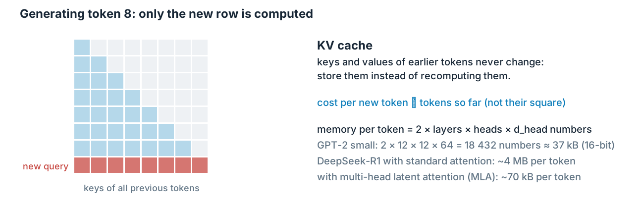
When a new token is generated only the last row of the attention pattern is new; keys and values of earlier tokens are stored in a cache

The full attention pattern has T2T^2 entries: a 100 000-token context compares every pair of words of a book. When generating, earlier keys and values do not change, so they are cached. The cache, not the weights, often limits how many users and how long a context a server can handle; DeepSeek’s multi-head latent attention compresses it 57-fold.

GPT-2 under the hood: marimo notebook

GPT2_under_the_hood.py:

  1. tokenize any text with three tokenizers
  2. next-token probabilities and generation
  3. attention pattern of any layer and head
  4. the logit lens for your prompt
  5. embedding neighbours and analogies
  6. timing with and without the KV cache
  7. a tiny GPT written from scratch, trained on the text of this course

From the Lecture_4A folder:

python3.12 -m venv .venv
.venv/bin/python -m pip install -r requirements.txt
.venv/bin/marimo edit GPT2_under_the_hood.py

CPU only; the first start downloads GPT-2 (~550 MB). The tiny GPT (0.8 M parameters) trains in about a minute.

Static export of the notebook

Beyond text

Anything that can be cut into tokens:

  • images: 16 × 16 pixel patches (Vision Transformer, 2020)
  • audio: short frames of a spectrogram (Whisper, 2022)
  • proteins: amino acids (AlphaFold 2, ESM)
  • particle physics: particles or detector hits in an event (jet tagging, tracking)

Shared embedding spaces connect them: CLIP maps images and captions to the same vectors.

2017 Transformer: attention is all you need

2018 GPT, BERT

2019 GPT-2: 1.5 B parameters

2020 GPT-3: 175 B; scaling laws; ViT

2022 ChatGPT

2024–25 reasoning models, open weights (Llama, DeepSeek-R1)

Summary

  1. Tokenizer: text → integers (BPE, trained once)
  2. Embedding: integers → vectors, plus position
  3. Attention: tokens read from each other, softmax(QK⊤/dk)V\operatorname{softmax}(QK^\top/\sqrt{d_k})V, causal in a decoder
  4. MLP: each token processed alone
  5. Blocks add to the residual stream, LL times
  6. Unembedding + softmax → next-token probabilities
  7. Sampling with temperature, repeat

Trained on one task, next-token prediction, with the cross-entropy, backpropagation and Adam of the previous lectures.

Lecture 4B: from a text predictor to a chat assistant and an agent: context windows, latency, “thinking”, tools and harnesses.

End

Thank you for the attention