Convolutional Neural Networks

How AlexNet learned to see

Mikhail Mikhasenko · Lecture 3B

Lecture 3B applies the networks of Lecture 3A to images. The storyline follows chapter 5 of “The Welch Labs Illustrated Guide to AI” (AlexNet): a kernel is a similarity template, layer-1 kernels are edge and colour detectors, activation maps are stacked and processed again, deeper layers respond to corners and eventually faces, and the last layers form an embedding space. All AlexNet figures are recomputed here from the pretrained torchvision weights by scripts/make_figures.py; the marimo notebook reproduces them live.

From numbers to pictures

A colour image is a tensor of pixel intensities: height × width × 3 channels (red, green, blue).

AlexNet reads a 224 × 224 × 3 tensor, 150 528 numbers, and returns 1000 probabilities, one per ImageNet class.

Inside there is nothing but the neurons of Lecture 3A: weighted sums, ReLUs, and a softmax at the end.

The new idea is how the weights are arranged.

224 × 224 × 3 → AlexNet →

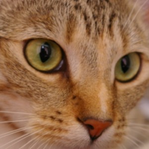
class	probability
Egyptian cat	0.80
tiger cat	0.13
tabby	0.07

Test image: “chelsea” from scikit-image (CC0). Probabilities from the torchvision AlexNet after resizing the short side to 256 and centre-cropping 224. The three most likely classes are all cats; ImageNet distinguishes several cat breeds.

MNIST: the classic benchmark

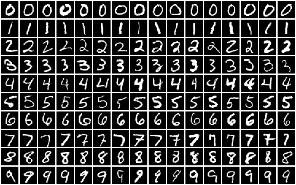
• 28 × 28 pixels, grey scale from 0 (black) to 255 (white)
• 60 000 training and 10 000 test images
• 10 classes: the digits 0–9
• Collected by LeCun, Cortes and Burges (1998) from US census and school handwriting

Small enough for a laptop, hard enough to separate methods.

The first 16 test images of each digit, drawn from the MNIST test set by scripts/make_figures.py. Original page: yann.lecun.com/exdb/mnist (web.archive.org copy). A classifier that ignores the image and always answers the same digit is right about 10% of the time.

MNIST: error rates

Model	Details	Test error
Linear classifier	pairwise, deskewed inputs	7.6 %
Random forest	fast unified random forests	2.8 %
Boosted stumps	on Haar features	0.87 %
Support-vector machine	degree-9 polynomial, jittered	0.56 %
Neural network	784–800–10, no distortions	1.6 %
Deep neural network	784–2500–2000–1500–1000–500–10, elastic distortions	0.35 %
Convolutional network	committee of 35 CNNs	0.23 %
Convolutional network	ensemble of 3 CNNs, augmentation	0.09 %

Dense networks need hand-made distortions to compete. Convolutional networks build in what images are like.

Selected rows of the table in the Wikipedia article “MNIST database” (the original lecture showed a screenshot of it); see the references there. Distortions and augmentation create shifted, rotated or elastically deformed training copies, which teaches a dense network the invariances that a CNN has by construction.

Why not a dense network?

Too many weights

One dense layer from a 224 × 224 × 3 image to 4096 units:

$$150\,528\times4096\approx6.2\times10^{8}\ \text{weights}$$

Wrong assumptions

A dense unit treats pixel 17 and pixel 17 000 as unrelated inputs. Shift the cat by a few pixels and every input changes.

What we know about images

Locality: nearby pixels belong together; an edge is a local pattern.

Translation: a pattern means the same thing anywhere in the image.

So: use small detectors, and apply the same detector at every position.

These two assumptions are the “inductive bias” of convolutional networks. They reduce the number of parameters enormously and make the output of a layer shift together with the input (translation equivariance). Pooling then adds some tolerance to small shifts.

A kernel is a template

Slide a small grid of weights, the kernel, over the image. At each position take the dot product of kernel and patch:

$$s=\sum_i w_i\,x_i=\lVert\mathbf w\rVert\,\lVert\mathbf x\rVert\cos\theta$$

Large when the patch looks like the kernel: a similarity score.

AlexNet kernel 9 (left) slid over an image that contains its own pattern, upright and rotated by 90°. Activation map (right): peak 9.0 on the upright copy, 0.0 on the rotated copy.

This reproduces the experiment in the Welch Labs guide (figure 5.8), where the author holds a printout of a first-layer kernel in front of the camera and the corresponding activation map lights up; rotating the paper by 90° weakens it. Here the patch is written in normalized input space as a tiled copy of the kernel, which maximizes the dot product for a given contrast. The map shown is conv1 followed by ReLU, 55 × 55, aligned with the input band.

Convolution

For one kernel $W$ of size $K\times K$, bias $b$, stride $S$ and padding $P$:

$$a_{ij}=h\!\left(b+\sum_{u=0}^{K-1}\sum_{v=0}^{K-1}W_{uv}\;x_{iS+u-P,\;jS+v-P}\right)$$

Output size for an $N\times N$ input:

$$N'=\left\lfloor\frac{N+2P-K}{S}\right\rfloor+1$$

• Local: each output looks at a $K\times K$ patch.
• Shared: the same $K^2+1$ numbers are used at every position.
• Stride $S$ skips positions; padding $P$ adds a border of zeros.

AlexNet conv1: $\lfloor(224+4-11)/4\rfloor+1=55$.

Deep-learning “convolution” does not flip the kernel; mathematicians call it cross-correlation.

With a flipped kernel the operation would be a true convolution; since the kernel is learned, the flip makes no difference. Padding “same” with K = 3 means P = 1 and keeps the size for stride 1. The next widget lets you change K’s weights, the stride and the padding.

Sliding a kernel over an image

Widget 1. Press Slide to animate the dot products. Compare the vertical and horizontal edge kernels on the digit 7 and on the square. Blur averages; sharpen enhances differences; identity reproduces the image. Switch on ReLU: only one side of each edge survives. Stride 2 halves the map; padding 1 keeps 28 × 28. Draw your own shapes (shift-drag erases). The classic Sobel kernels here were designed by hand; in a CNN these numbers are learned.

Channels: stack and repeat

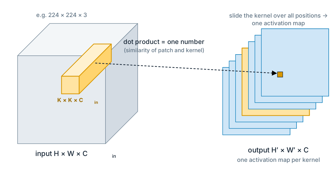
A kernel always spans all input channels: $K\times K\times C_{\mathrm{in}}$ weights.

$C_{\mathrm{out}}$ kernels give $C_{\mathrm{out}}$ activation maps. Stacked, they form a new tensor $H'\times W'\times C_{\mathrm{out}}$.

The next layer processes it exactly like an image, only with $C_{\mathrm{out}}$ “colours”.

Parameters: $K^2\,C_{\mathrm{in}}\,C_{\mathrm{out}}+C_{\mathrm{out}}$.

AlexNet conv1 has 64 kernels of 11 × 11 × 3 and produces 64 maps of 55 × 55. conv2 then uses 192 kernels of 5 × 5 × 64. This is “stack and repeat” in the Welch Labs guide (figure 5.9): after the first layer the same operation is simply applied again with different learned weights.

Counting parameters

	Weights	Share of AlexNet
conv1: 64 kernels of 11 × 11 × 3, plus biases	23 296
a dense layer with the same 55 × 55 × 64 outputs	$2.9\times10^{10}$
all 5 convolutional layers	2.5 M	4 % of weights, 92 % of computation
the 3 dense layers	58.6 M	96 % of weights, 8 % of computation

Weight sharing cuts conv1 by a factor of a million. The convolutional layers are cheap to store but expensive to run: every weight is used at thousands of positions.

Numbers for the torchvision AlexNet (61.1 M parameters in total). Computation counted as multiply–accumulate operations for one 224 × 224 image: 0.66 billion in the convolutional layers, 0.06 billion in the dense layers. The dense alternative to conv1 would connect 150 528 inputs to 193 600 outputs.

Pooling

Max pooling keeps the largest value in each window:

1	3	2	0
4	2	1	5
0	1	3	2
2	6	1	0

→

4	5
6	3

2 × 2 window, stride 2: a quarter of the values survive.

• Smaller maps: less computation in later layers.
• Tolerance to small shifts: the maximum barely moves.
• Larger receptive fields: later kernels see more of the image.

No weights to learn. AlexNet uses overlapping 3 × 3 windows with stride 2.

Average pooling takes the mean instead. Modern networks often replace pooling by convolutions with stride 2, and end with global average pooling over the whole map. The next widget combines conv → ReLU → max-pool → conv.

Stack and repeat: from edges to corners

Widget 2. The four layer-1 kernels detect top, bottom, left and right edges of a dark shape. After ReLU and 2 × 2 max pooling, the four maps are stacked. Each layer-2 kernel has 3 × 3 × 4 weights: for the top-left corner it adds the top-edge map to the right of the centre and the left-edge map below it; the bias −1.2 means one edge alone is not enough. Hover a corner map to see its 8 × 8 receptive field. On the square, each corner type fires exactly once; on the triangle, only the two base corners fire strongly. These weights are hand-set; AlexNet’s conv2 learned such detectors from data (next slides).

A convolutional network

Blocks

$\big[\,\text{conv}\to\text{ReLU}\to\text{pool}\,\big]\times n\ \to$ flatten $\to$ dense layers $\to$ softmax

Features first, then a classifier: the dense end is the MLP of Lecture 3A.

LeNet-5 (LeCun et al., 1998)

32 × 32 digit → 6 maps 28 × 28 → pool → 16 maps 10 × 10 → pool → 120 → 84 → 10. About 60 000 parameters; read bank cheques in the 1990s.

Receptive fields grow

AlexNet layer	pixels seen by one unit
conv1	11 × 11
conv2	51 × 51
conv3	99 × 99
conv5	163 × 163

Deep units see large parts of the 224 × 224 image.

Receptive field recursion: r_l = r_(l−1) + (K_l − 1) · j_(l−1), where j is the product of all previous strides. AlexNet: conv1 11 (j = 4), pool 19 (j = 8), conv2 51, pool 67 (j = 16), conv3 99, conv4 131, conv5 163, pool 195. The effective receptive field, where the unit is actually sensitive, is smaller and concentrated in the centre.

Train a network, then draw for it

The widget runs the forward pass of the CNN in the browser; the weights after 0, 1, 2 and 3 epochs were trained in Julia (Flux) by scripts/make_mnist_data.jl on all 60 000 training digits (Adam, batches of 128). The same network lives in pluto/mnist-draw.jl for training it live: make -C slides start-julia-server DECK=Lecture_3B.

Suggested sequence: pick “untrained” and draw a digit (random guess, test accuracy about 10 %). Switch to 1 epoch: about 96 %. Draw again; ask the audience for hard digits (a 4 with an open top, a 7 with a bar, a 1 with a foot). Watch the layer-1 maps: edge and stroke detectors, the same 8 filters applied everywhere. Only 5 258 weights, against about 100 000 for a dense 784–128–10 network.

The pad crops the drawing, scales it into 20 × 20 and centres it by its centre of mass in 28 × 28, as the MNIST digits were prepared. After clicking into the widget, click the slide title to get the arrow keys back.

Shift the digits

MNIST digits are centred. Move every test image a few pixels to the right and measure again.

shift	0 px	2 px	3 px
dense 784–128–10	96 %	75 %	47 %
boosted trees (JLBoost)	90 %	69 %	51 %
CNN	97 %	91 %	74 %

Trees and dense networks see each pixel as a fixed input. The CNN applies the same kernels everywhere and pools.

The widget shows the CNN of the previous slide after 3 epochs on a shifted test digit, and the accuracy curves of the CNN and the dense network (both 3 epochs, from scripts/make_mnist_data.jl). The table was measured offline on 2 000 test images, networks trained for 3 epochs; the trees are ten one-versus-rest JLBoost boosters (10 000 images, 20 rounds, depth 4, 92 % unshifted), see pluto/mnist-trees.jl and pluto/README.md. This is the “shift the cat” argument of the “Why not a dense network?” slide, measured. Pooling gives only limited invariance, so the CNN also degrades for larger shifts; data augmentation (shifted training copies) fixes the rest.

ImageNet

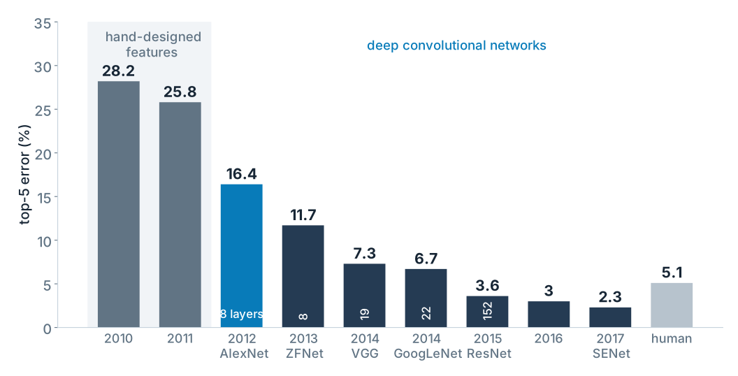
ILSVRC 2010–2017: 1.2 million training images, 1000 classes. Score: top-5 error, the fraction of images whose true class is not among the five best guesses.

Before 2012: hand-designed features (SIFT, Fisher vectors) and linear classifiers.

2012, AlexNet (Krizhevsky, Sutskever, Hinton): 16.4 %, against 26.2 % for the runner-up.

After 2012 every winner was a deep convolutional network.

Numbers as in Stanford CS231n. AlexNet’s paper reports 15.3% for its best entry, which also used extra pre-training data; 16.4% averages five CNNs trained on ILSVRC data only. The runner-up in 2012 (26.2%) used hand-designed features. The human estimate of 5.1% (Russakovsky et al. 2015) comes from one trained annotator. The original lecture also showed the error rates of all entries per year.

AlexNet

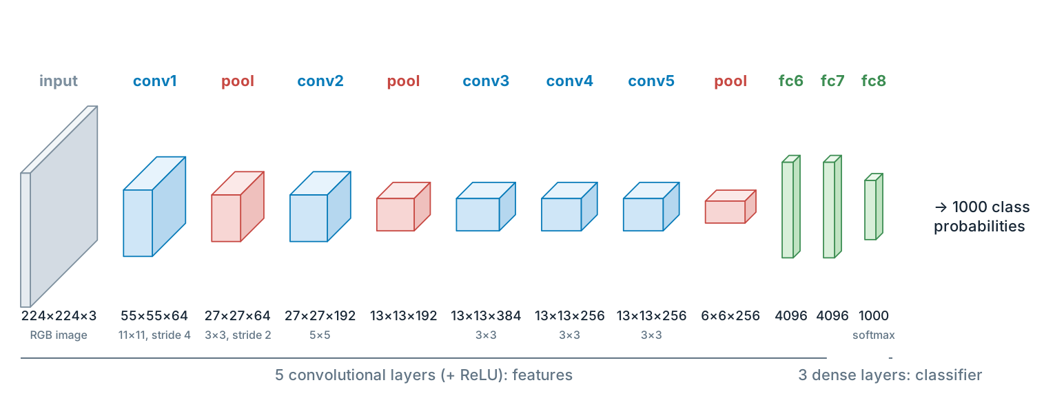
(CONV → RN → MP)² → CONV³ → MP → (FC → DO)² → Linear → softmax

CONV: convolution + ReLU · RN: local response normalization · MP: max pooling · FC: dense + ReLU · DO: dropout

Shapes are those of the torchvision AlexNet used for all figures and the notebook (64, 192, 384, 256, 256 kernels; no response normalization). The 2012 original had 96, 256, 384, 384, 256 kernels, split across two GPUs that only exchanged data in some layers, and local response normalization (RN) after conv1 and conv2. The prisms show the data tensors flowing through the network, not the operations.

What made AlexNet work

• ReLU activations: several times faster training than tanh
• Dropout (p = 0.5) in the two big dense layers
• Data augmentation: random 224 × 224 crops of 256 × 256 images, horizontal flips, colour shifts
• SGD with momentum 0.9, weight decay 0.0005, batch 128

• Two GTX 580 GPUs (3 GB each), five to six days of training
• 60 million parameters, 650 000 neurons
• ImageNet: the first labelled image set large enough to feed such a model

The algorithms were from the 1980s. The scale of data and compute was new.

Krizhevsky, Sutskever & Hinton, “ImageNet Classification with Deep Convolutional Neural Networks”, NeurIPS 2012. They report that a four-layer CNN with ReLUs reached 25% training error on CIFAR-10 six times faster than the same network with tanh. Ilya Sutskever later co-founded OpenAI. Dropout, momentum and weight decay are the tools of Lecture 3A.

Layer 1: what did AlexNet learn?

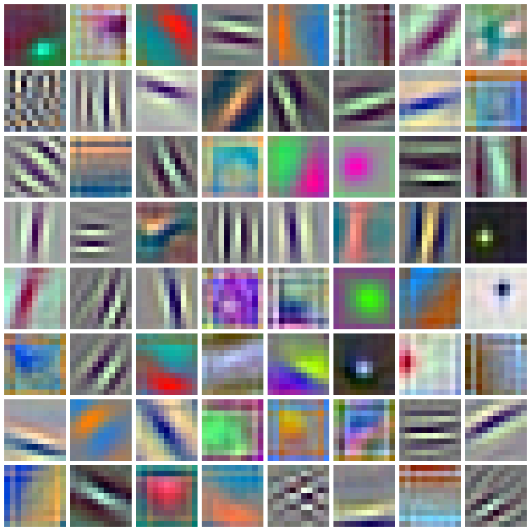
Each first-layer kernel has depth 3, like the image, so it is a tiny RGB picture.

• edge detectors at many angles and frequencies
• colour blobs and colour-opponent edges

Every kernel started as random numbers. These patterns were learned from labelled photos alone.

The 64 kernels of the torchvision AlexNet, each rescaled to its own minimum and maximum. Similar Gabor-like filters are found in the primary visual cortex of mammals. In the original two-GPU AlexNet one GPU specialized in black-and-white edge detectors and the other in colour blobs (Welch Labs guide, footnote to figure 5.7).

Activation maps

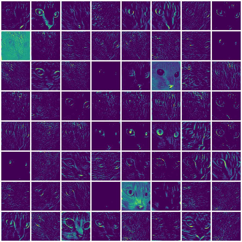
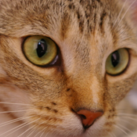
Sliding each of the 64 kernels over the photo gives 64 activation maps (55 × 55 after ReLU).

A map is bright where the image looks like its kernel: whiskers, eye outlines, fur texture, the pink nose.

Maps are shown with the viridis colour scale, each normalized to its own maximum. Several maps respond mainly to colour (for example the nose or the green eyes), others to edges at particular orientations.

Layer 2: combining edges

input: a sheet of paper

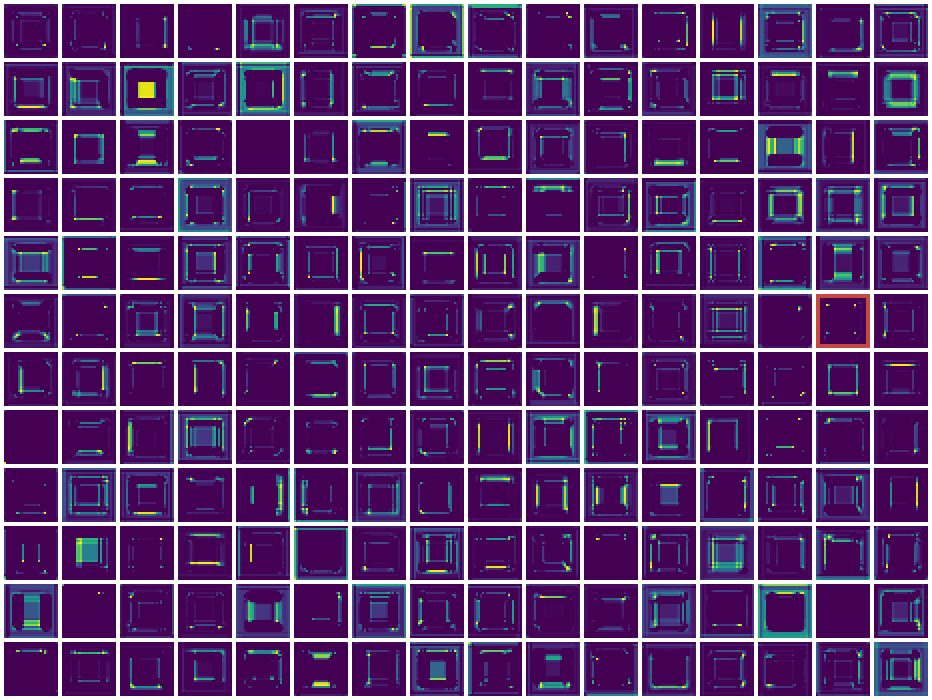
all 192 conv2 maps

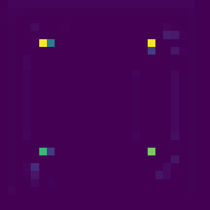
channel 94: corners

Layer-2 kernels are 5 × 5 × 64: we cannot draw them, but we can watch what they respond to. Most maps trace edges of the square; channel 94 fires almost only at its corners.

Reproduces the “corner detector” observation of the Welch Labs guide (figure 5.10; their feature map 104 was found on a photo of a sheet of paper). Here the input is a synthetic white square and channel 94 of the torchvision conv2 lights up at three corners and part of the right edge. Compare with the hand-built corner detector of widget 2.

Layer 5: a face detector nobody asked for

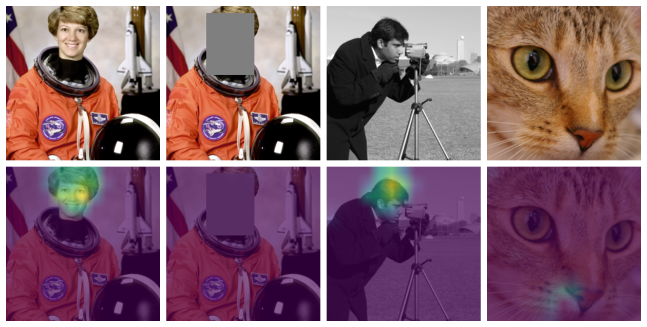
conv5, channel 174 · peak activation 14.5 on the astronaut’s face, 0.8 with the face covered, 14.5 on the cameraman, 5.8 on the cat’s nose. ImageNet has no “face” or “person” class.

Maps are 13 × 13, upsampled and overlaid on the input, with one shared colour scale. The Welch Labs guide found such a unit (their activation map 186) with a webcam; with these test images the face unit of the torchvision AlexNet is channel 174. A plausible explanation: many ImageNet classes are photographed together with people (dumbbells, microphones, seat belts), so a face detector is a useful intermediate concept.

What does a unit want to see?

conv1 · 9
stripesconv2 · 94
cornersconv3 · 150conv4 · 60conv5 · 174
eyes, nosefc8 · goldfish

Start from noise and change the image by gradient ascent until one unit is as active as possible; the weights stay fixed. Deeper units prefer textures, patterns, object parts.

Feature visualization: Erhan et al. (2009), Olah, Mordvintsev & Schubert, “Feature Visualization”, Distill (2017). Regularizers here are random shifts of the image and a small blur every eight steps; better methods use Fourier parametrization and transformations and produce cleaner images, as in the Welch Labs guide’s figure 5.14 (InceptionV1). Activation atlases (Carter et al., Distill 2019) combine such images with a 2D map of the embedding space.

What AlexNet says, and why

image	top prediction
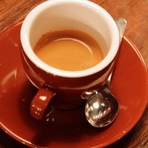	espresso 0.97
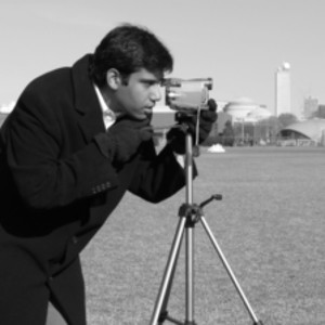	tripod 0.72
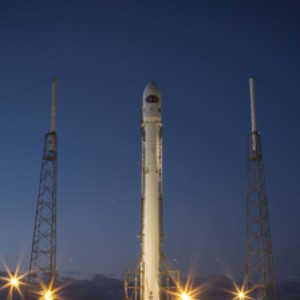	mosque 0.63
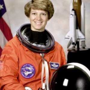	dumbbell 0.27

There is no “rocket” or “astronaut” class. A classifier always picks one of its labels.

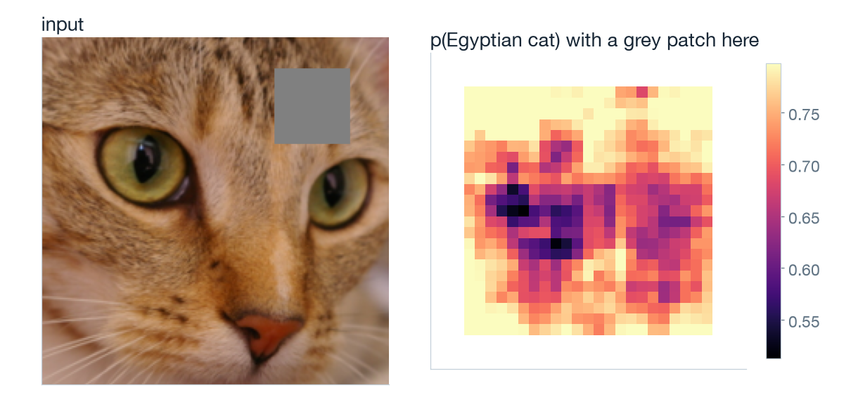
Occlusion: grey out a patch, record p(Egyptian cat). Covering the eyes hurts most (0.80 → 0.51).

Occlusion sensitivity: Zeiler & Fergus (2014). A 48 × 48 grey patch is moved with stride 8; each pixel of the map is one forward pass (23 × 23 = 529 passes). The notebook runs this for any image and patch size.

The embedding space

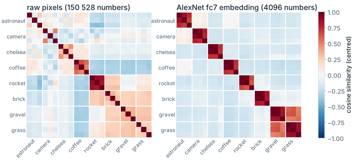
Stop before the classifier: every image becomes a point in a 4096-dimensional space (fc7). Flipped and cropped copies of the same photo: similarity 0.34 in pixels, 0.83 in the embedding.

Cosine similarity after subtracting the mean vector of the 24 images. The AlexNet paper showed that nearest neighbours of a test image in this space show the same kind of object, although their pixels are very different. Word embeddings in language models behave the same way (the classic example: king − man + woman ≈ queen). Embeddings are the bridge from AlexNet to modern language models, where every token is mapped to such a vector.

AlexNet under the hood: marimo notebook

AlexNet_under_the_hood.py loads the pretrained network and lets you

1. classify the samples or your own photo
2. browse the 64 layer-1 kernels and their maps
3. open the activation maps of any layer and channel
4. run the occlusion experiment
5. visualize what a unit wants to see
6. place your image in the embedding space

From the Lecture_3B folder:

python3.12 -m venv .venv
.venv/bin/python -m pip install -r requirements.txt
.venv/bin/marimo edit AlexNet_under_the_hood.py

Runs on a laptop CPU; the first start downloads the weights (~240 MB).

Static export of the notebook

Suggested live demo: upload a selfie, look at conv5 channel 174, then cover your face with your hand. Try the printed-kernel experiment of the Welch Labs guide with a phone photo. The static export shows the default outputs; interactive controls need the running notebook. The same figures for the slides come from scripts/make_figures.py.

After AlexNet: deeper

VGG (2014): only 3 × 3 kernels, 16–19 layers. Two 3 × 3 layers see 5 × 5 with fewer weights.

GoogLeNet (2014): 22 layers of parallel “inception” branches.

ResNet (2015): 152 layers, 3.6 % top-5 error. Each block learns a correction to its input: $$\mathbf y=\mathbf x+F(\mathbf x)$$

The skip connection gives gradients a direct path back through many layers: the vanishing-gradient problem of Lecture 3A, solved by architecture.

Since 2020, vision transformers cut images into patches and treat them like words, using the same blocks as language models. Their “Add & Norm” is ResNet’s skip connection.

Simonyan & Zisserman (2014), Szegedy et al. (2014), He et al., “Deep Residual Learning”, arXiv:1512.03385. Dosovitskiy et al., “An Image is Worth 16x16 Words” (2020). Batch normalization (Lecture 3A) made these depths trainable too. The original lecture’s VGG-16 diagram is replaced by this summary.

Scale

	LeNet-5	AlexNet	GPT-3
Year	1998	2012	2020
Data	MNIST: 60 000 images, 10 classes	ImageNet: 1.2 M images, 1000 classes	~300 billion tokens of text
Compute	one CPU	two gaming GPUs	thousands of data-centre GPUs
Parameters	~60 000	~60 million	175 billion
Layers	5	8	96
Key parts	convolutions, tanh	convolutions, ReLU, dropout	transformer blocks with dense layers

The same building blocks, scaled up by factors of a thousand at every step.

After the comparison figure in chapter 5 of the Welch Labs guide. GPT-3 numbers from Brown et al. (2020): 175 B parameters, 96 layers, trained on about 300 B tokens. Hinton’s group in 2012 had roughly ten thousand times the compute LeCun had fifteen years earlier. Scale of data and compute, more than new algorithms, drove the 2012 breakthrough; whether scale alone continues to work is an open question.

End

Thank you for the attention