Neural Networks

From one neuron to deep networks

Mikhail Mikhasenko · Lecture 3A

Where we are

The recipe from Lecture 1B
  1. A model f(x;θ)f(x;\theta) with parameters θ\theta
  2. A loss L(θ)L(\theta) that measures mistakes on training data
  3. An optimizer that lowers L(θ)L(\theta)

Trees (2A, 2B): piecewise-constant models grown by greedy cuts.

Today

Neural networks are smooth functions with many parameters, fitted by following the gradient of the loss.

  • What does a network compute?
  • Why do we need hidden layers and nonlinearities?
  • How do we compute gradients efficiently, and which way do we step?

Origins

1943 McCulloch & Pitts: a binary-threshold neuron model

1949 Hebb: connections that fire together strengthen

1958 Rosenblatt: the perceptron learns weights from labelled examples (Mark I Perceptron: 20 × 20 photocell images)

1969 Minsky & Papert, Perceptrons: the limits of one layer
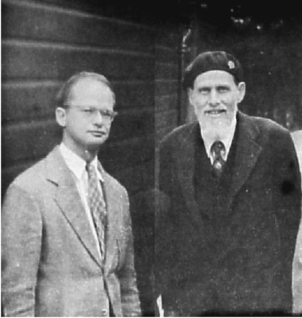
Warren McCulloch and Walter Pitts, Chicago 1949

Warren McCulloch and Walter Pitts, Chicago 1949

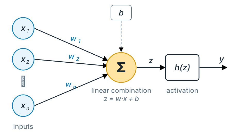
The artificial neuron

y=h(∑i=1nwixi+b)=h(𝐰⋅𝐱+b)y=h\!\left(\sum_{i=1}^{n}w_i x_i+b\right)=h(\mathbf w\cdot\mathbf x+b)

  • weights wiw_i: how strongly each input counts
  • bias bb: shifts the threshold
  • activation hh: a fixed nonlinear function

An affine map followed by a nonlinearity. The perceptron uses a step: h(z)=1h(z)=1 if z≥0z\ge 0, else 00.

Inputs x1 to xn, multiplied by weights w1 to wn, summed with bias b into z, passed through the activation h to give the output y

One neuron, one line

Geometry

The boundary 𝐰⋅𝐱+b=0\mathbf w\cdot\mathbf x+b=0 is a straight line (a hyperplane in nn dimensions).

  • 𝐰\mathbf w is normal to the line and points towards z>0z>0.
  • bb moves the line: its distance from the origin is |b|/‖𝐰‖|b|/\lVert\mathbf w\rVert.
  • For a sigmoid, larger ‖𝐰‖\lVert\mathbf w\rVert makes the transition sharper.
Perceptron learning rule

For each example, with prediction ŷ∈{0,1}\hat y\in\{0,1\}:

𝐰←𝐰+η(y−ŷ)𝐱,b←b+η(y−ŷ)\mathbf w\leftarrow\mathbf w+\eta\,(y-\hat y)\,\mathbf x,\qquad b\leftarrow b+\eta\,(y-\hat y)

Correct predictions change nothing; a mistake tilts the line towards the misclassified point.

If a separating line exists, the rule finds one in a finite number of steps.

One neuron draws one line

The XOR problem and the first AI winter

1969: Minsky and Papert prove that a single-layer perceptron cannot compute some simple functions, for example XOR.

x1x_1 x2x_2 XOR
0 0 0
0 1 1
1 0 1
1 1 0

No single line separates the ones from the zeros. Funding and interest in neural networks declined through the 1970s.
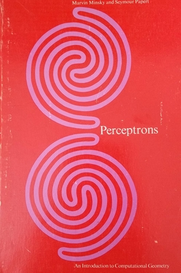
Cover of Perceptrons by Marvin Minsky and Seymour Papert

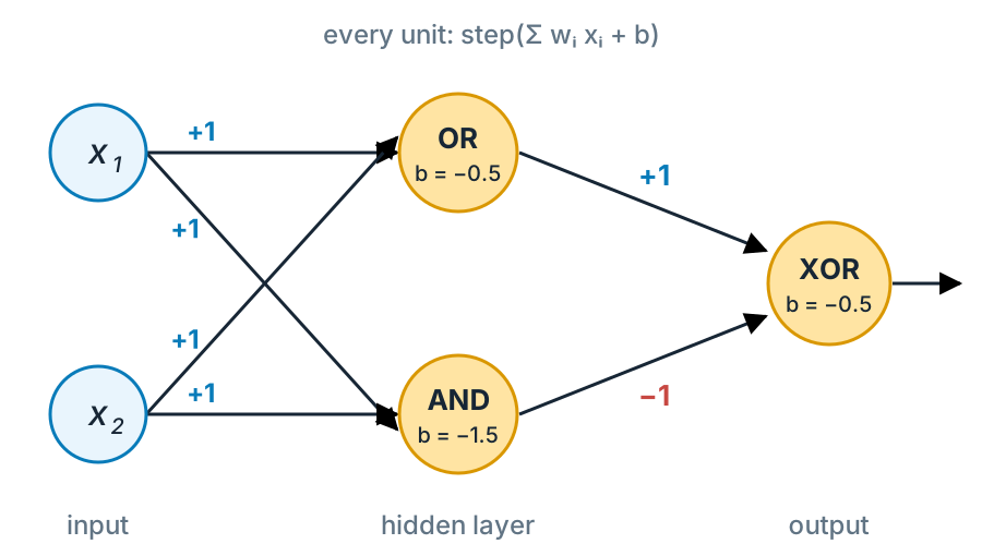
One hidden layer solves XOR

A 2-2-1 network: hidden units OR and AND, output computes OR and not AND

x1x_1 x2x_2 OR AND OR − AND
0 0 0 0 0
0 1 1 0 1
1 0 1 0 1
1 1 1 1 0

The hidden units compute new features. In the (OR, AND) plane, XOR is separable by one line.

Multilayer perceptron

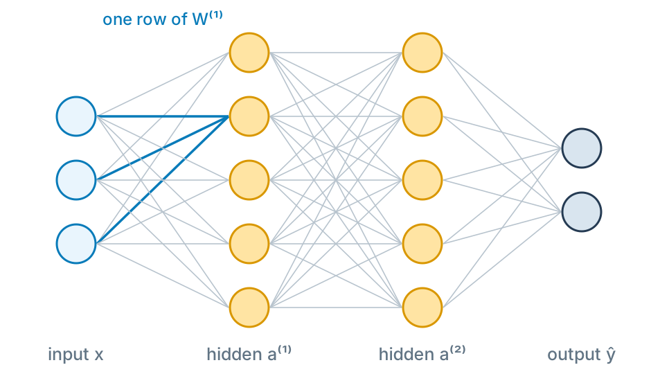
Stack layers of neurons. With 𝐚(0)=𝐱\mathbf a^{(0)}=\mathbf x:

𝐚(l)=h(W(l)𝐚(l−1)+𝐛(l)),l=1,…,L\mathbf a^{(l)}=h\!\left(W^{(l)}\mathbf a^{(l-1)}+\mathbf b^{(l)}\right),\qquad l=1,\dots,L

W(l)W^{(l)} has shape nl×nl−1n_l\times n_{l-1}: each row holds the weights of one unit.

Dense (fully connected): every unit sees every unit of the previous layer.

Example, MNIST 784–800–10: 784⋅800+800+800⋅10+10=636010784\cdot800+800+800\cdot10+10=636\,010 parameters.

A network with 3 inputs, two hidden layers of 5 units and 2 outputs; the weights into one hidden unit are highlighted

Why the nonlinearity?

Without hh, two layers collapse into one:

W(2)(W(1)𝐱+𝐛(1))+𝐛(2)=W(2)W(1)⏟W𝐱+W(2)𝐛(1)+𝐛(2)⏟𝐛W^{(2)}\!\left(W^{(1)}\mathbf x+\mathbf b^{(1)}\right)+\mathbf b^{(2)} =\underbrace{W^{(2)}W^{(1)}}_{W}\mathbf x+\underbrace{W^{(2)}\mathbf b^{(1)}+\mathbf b^{(2)}}_{\mathbf b}

Any depth of linear layers is still one linear map: one line, no XOR.

The activation bends the space between layers. Composing many simple bends builds complicated functions.

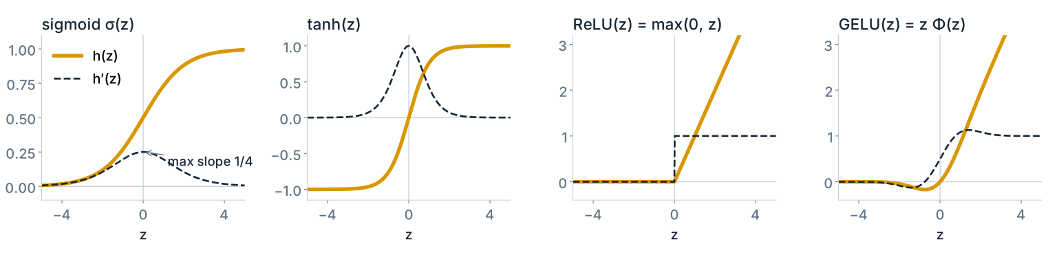
Activation functions

Sigmoid, tanh, ReLU and GELU with their derivatives

Sigmoid, tanh saturate: σ′(z)≤14\sigma'(z)\le\tfrac14. Ten layers can shrink a gradient by 4−10≈10−64^{-10}\approx10^{-6} (vanishing gradient). Still used for outputs and gates.
ReLU max(0,z)\max(0,z): cheap, slope 1 for z>0z>0. Units stuck at z<0z<0 stop learning (“dying ReLU”); leaky ReLU keeps a small slope.
GELU zΦ(z)z\,\Phi(z), Φ\Phi = Gaussian CDF: a smooth ReLU, standard in transformers (BERT, GPT-2).

Universal approximation

1989, Cybenko: one hidden layer is enough. For a sigmoidal σ\sigma, any continuous ff on a bounded domain and any ε>0\varepsilon>0 there exist NN and parameters with

g(𝐱)=∑j=1Nvjσ(𝐰j⊤𝐱+bj),|g(𝐱)−f(𝐱)|<ε.g(\mathbf x)=\sum_{j=1}^{N}v_j\,\sigma\!\left(\mathbf w_j^{\top}\mathbf x+b_j\right),\qquad |g(\mathbf x)-f(\mathbf x)|<\varepsilon .

Hornik (1991), Leshno et al. (1993): any non-polynomial activation works, including ReLU.

What it does not say
  • how large NN must be (it can grow exponentially with dimension)
  • how to find the weights
  • how well gg generalizes beyond the training data

In practice, deep networks reach the same accuracy with far fewer units than one wide layer.

Universal approximation: the visual proof

Your turn: build a shape from ReLUs

Four hidden ReLU units, no output bias:

y=∑j=14vjrelu(wjx+bj)y=\sum_{j=1}^{4}v_j\,\mathrm{relu}(w_j x+b_j)

Each unit adds one kink at x=−bj/wjx=-b_j/w_j, where the slope changes by vjwjv_j w_j.

Task
  1. A triangle: 00 outside [−1,1][-1,1], peak 11 at x=0x=0
  2. A trapezium: flat top 11 on [−1,1][-1,1], down to 00 at ±2\pm2
Sliders: w1…4w_{1\ldots4}, b1…4b_{1\ldots4}, vj=w4+jv_j=w_{4+j}. Live Julia (Flux + Plots) via Pluto.

Output layers and losses

Task Output unit Loss
Regression identity: ŷ=z\hat y=z squared error 12(ŷ−y)2\tfrac12(\hat y-y)^2
Binary classification sigmoid p̂=σ(z)\hat p=\sigma(z) cross-entropy −ylogp̂−(1−y)log(1−p̂)-y\log\hat p-(1-y)\log(1-\hat p)
KK classes softmax pk=ezk∑jezj\displaystyle p_k=\frac{e^{z_k}}{\sum_{j}e^{z_j}} cross-entropy −logpy-\log p_{y}
Positive quantity softplus log(1+ez)\log(1+e^{z}) e.g. Gaussian negative log-likelihood

For sigmoid or softmax with cross-entropy, the gradient at the output is simply ∂L/∂zk=pk−𝟙[k=y]\partial L/\partial z_k=p_k-\mathbb 1[k=y].

Gradient descent

The loss averages over NN training examples:

L(θ)=1N∑i=1Nℓ(f(xi;θ),yi)L(\theta)=\frac1N\sum_{i=1}^{N}\ell\big(f(x_i;\theta),\,y_i\big)

Step against the gradient:

θn+1=θn−η∇θL(θn)\theta_{n+1}=\theta_n-\eta\,\nabla_{\theta}L(\theta_n)

η\eta is the learning rate.

Like walking downhill in the dark with a flashlight: you only see the slope at your feet.

Near a minimum with curvature λ\lambda the error is multiplied by 1−ηλ1-\eta\lambda at every step:

  • ηλ<1\eta\lambda<1: smooth approach
  • 1<ηλ<21<\eta\lambda<2: zig-zag, still converges
  • ηλ>2\eta\lambda>2: diverges

Choosing the learning rate

Backpropagation: the chain rule on a graph
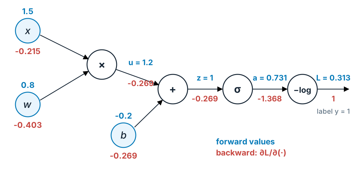
Computational graph of a sigmoid neuron with cross-entropy loss, with forward values and backward gradients

∂L∂w=−1a⏟∂L/∂a⋅a(1−a)⏟∂a/∂z⋅1⏟∂z/∂u⋅x⏟∂u/∂w=(a−y)x=−0.403\frac{\partial L}{\partial w}= \underbrace{-\frac1a}_{\partial L/\partial a}\cdot \underbrace{a(1-a)}_{\partial a/\partial z}\cdot \underbrace{1}_{\partial z/\partial u}\cdot \underbrace{x}_{\partial u/\partial w} =(a-y)\,x=-0.403

Forward: compute and store every intermediate value. Backward: multiply local derivatives from the loss towards the inputs.

Backpropagation through layers

Define the error signal 𝛅(l)=∂L/∂𝐳(l)\boldsymbol\delta^{(l)}=\partial L/\partial\mathbf z^{(l)}, where 𝐳(l)=W(l)𝐚(l−1)+𝐛(l)\mathbf z^{(l)}=W^{(l)}\mathbf a^{(l-1)}+\mathbf b^{(l)}:

𝛅(L)=𝐩̂−𝐲,𝛅(l)=(W(l+1)⊤𝛅(l+1))⊙h′(𝐳(l))\boldsymbol\delta^{(L)}=\hat{\mathbf p}-\mathbf y,\qquad \boldsymbol\delta^{(l)}=\left(W^{(l+1)\top}\boldsymbol\delta^{(l+1)}\right)\odot h'\!\left(\mathbf z^{(l)}\right)

∂L∂W(l)=𝛅(l)𝐚(l−1)⊤,∂L∂𝐛(l)=𝛅(l)\frac{\partial L}{\partial W^{(l)}}=\boldsymbol\delta^{(l)}\,\mathbf a^{(l-1)\top},\qquad \frac{\partial L}{\partial\mathbf b^{(l)}}=\boldsymbol\delta^{(l)}

One backward pass costs about as much as one forward pass, whether the network has ten parameters or ten billion.

1970 Linnainmaa: reverse-mode automatic differentiation

1974 Werbos: applied to neural networks

1986 Rumelhart, Hinton & Williams: rediscovered and popularized

Nobel Prize medal

2024 Nobel Prize in Physics, Hopfield & Hinton: “for foundational discoveries and inventions that enable machine learning with artificial neural networks”

Mini-batches: stochastic gradient descent

With N=106N=10^6 examples, the exact gradient is expensive. Estimate it on a random batch BB of mm examples (m≈32m\approx 32–512512):

𝐠=1m∑i∈B∇θℓi,𝔼[𝐠]=∇θL\mathbf g=\frac1m\sum_{i\in B}\nabla_\theta\,\ell_i,\qquad \mathbb E[\mathbf g]=\nabla_\theta L

The loss being minimized changes a little every step. One pass over all data is an epoch.

With a batch dimension the input is a matrix XX of shape m×dm\times d:

Z(1)=XW(1)⊤+𝟏𝐛(1)⊤Z^{(1)}=X\,W^{(1)\top}+\mathbf 1\,\mathbf b^{(1)\top}

Every layer is one matrix multiplication, which GPUs execute very fast.

Gradient noise shrinks like 1/m1/\sqrt m, and a little noise can help escape saddle points and sharp minima.

Momentum

Keep the inertia of the motion:

𝐯n=β𝐯n−1+𝐠n,θn+1=θn−η𝐯n\mathbf v_n=\beta\,\mathbf v_{n-1}+\mathbf g_n,\qquad \theta_{n+1}=\theta_n-\eta\,\mathbf v_n

Unrolled, 𝐯n=∑k≥0βk𝐠n−k\mathbf v_n=\sum_{k\ge0}\beta^k\,\mathbf g_{n-k}: an exponentially decaying memory of past gradients, about 1/(1−β)=101/(1-\beta)=10 steps for β=0.9\beta=0.9.

  • Consistent directions add up: up to 1/(1−β)1/(1-\beta) times faster.
  • Oscillating directions cancel: less zig-zag.
  • Speed can carry the parameters through small bumps and plateaus.

Polyak’s “heavy ball” (1964).

Adaptive step sizes: AdaGrad and RMSProp

Give every parameter its own step size. Per coordinate:

sn={sn−1+gn2AdaGradβ2sn−1+(1−β2)gn2RMSProps_n=\begin{cases}s_{n-1}+g_n^2 & \text{AdaGrad}\\[2pt] \beta_2\,s_{n-1}+(1-\beta_2)\,g_n^2 & \text{RMSProp}\end{cases}

θn+1=θn−ηgnsn+ε\theta_{n+1}=\theta_n-\eta\,\frac{g_n}{\sqrt{s_n}+\varepsilon}

  • Steep directions get small steps; flat ones get relatively large steps.
  • Rarely updated parameters (sparse features) catch up instead of being left behind.
  • AdaGrad’s sns_n only grows, so its steps shrink towards zero. RMSProp forgets old gradients.

Adam: adaptive moment estimation

𝐦n=β1𝐦n−1+(1−β1)𝐠n,𝐬n=β2𝐬n−1+(1−β2)𝐠n2\mathbf m_n=\beta_1\mathbf m_{n-1}+(1-\beta_1)\,\mathbf g_n,\qquad \mathbf s_n=\beta_2\mathbf s_{n-1}+(1-\beta_2)\,\mathbf g_n^2

𝐦̂n=𝐦n1−β1n,𝐬̂n=𝐬n1−β2n,θn+1=θn−η𝐦̂n𝐬̂n+ε\hat{\mathbf m}_n=\frac{\mathbf m_n}{1-\beta_1^n},\qquad \hat{\mathbf s}_n=\frac{\mathbf s_n}{1-\beta_2^n},\qquad \theta_{n+1}=\theta_n-\eta\,\frac{\hat{\mathbf m}_n}{\sqrt{\hat{\mathbf s}_n}+\varepsilon}

Defaults: η=10−3\eta=10^{-3}, β1=0.9\beta_1=0.9, β2=0.999\beta_2=0.999, ε=10−8\varepsilon=10^{-8}.

Momentum (first moment 𝐦\mathbf m): speed along consistent directions

RMSProp (second moment 𝐬\mathbf s): per-parameter step sizes

Bias correction: 𝐦\mathbf m and 𝐬\mathbf s start at zero

The default choice for most networks today, often as AdamW with decoupled weight decay.

Optimizers on a loss surface

Initialization

Break the symmetry

If all weights start equal, all units in a layer compute the same function and receive the same gradient, forever. Start with 𝐛=0\mathbf b=0 and random WW.

Choose the scale

For z=∑i=1ninwiaiz=\sum_{i=1}^{n_{\mathrm{in}}}w_i a_i with independent terms, Varz=ninVarwVara\operatorname{Var}z=n_{\mathrm{in}}\operatorname{Var}w\,\operatorname{Var}a. Keep the variance of signals and gradients constant from layer to layer.

Tanh, sigmoid: Glorot (Xavier), 2010

Varw=2nin+nout,w∼U(±6nin+nout)\operatorname{Var}w=\frac{2}{n_{\mathrm{in}}+n_{\mathrm{out}}},\quad w\sim U\!\left(\pm\sqrt{\tfrac{6}{n_{\mathrm{in}}+n_{\mathrm{out}}}}\right)

ReLU: He (Kaiming), 2015

w∼𝒩(0,2nin)w\sim\mathcal N\!\left(0,\ \frac{2}{n_{\mathrm{in}}}\right)

ReLU zeroes half the signal, hence the factor 2.

Overfitting and regularization

A large network can memorize the training data, noise included (bias and variance, Lecture 2A).

  • Validation set and early stopping: stop when the validation loss rises.
  • L2 / weight decay: minimize L+λ2‖θ‖2L+\tfrac{\lambda}{2}\lVert\theta\rVert^2; penalizes large weights (1990s).
  • More data, data augmentation: shifted, flipped, cropped copies (Lecture 3B).
  • Dropout (2012): during training, set each hidden unit to zero with probability pp. Like averaging many thinned networks.
  • Batch normalization (2015): normalize each unit over the batch, then learn a scale and a shift. Mainly stabilizes and speeds up training.
  • Ensembles: average independently trained networks.

Train a small network

The deep-learning renaissance

2009 Training on GPUs

2010 Glorot & Bengio: why deep networks were hard to train, better initialization

2011–12 ReLU and dropout

2012 AlexNet wins ImageNet by a wide margin

2015 Deep networks dominate vision, speech and language benchmarks

Next lecture: how convolutional networks see.
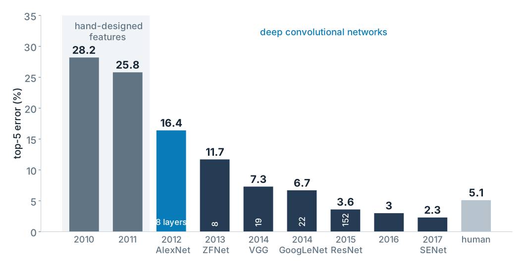
ImageNet challenge top-5 error of the winning entries, 2010 to 2017, compared with a human estimate

End

Thank you for the attention