Gradient Boosting

Decision trees, one correction at a time

Mikhail Mikhasenko · Lecture 2B

Continues Lecture 2A, which introduced trees, bagging and AdaBoost. This lecture builds gradient-boosted decision trees (BDTs) for regression with MSE and for classification with binary cross-entropy. Three questions guide the lecture: how a split is chosen, how leaf values are computed, and how the trees are combined.

AdaBoost recap

Iterative error correction with weak learners.

• Each new tree sees the same events, reweighted.
• Misclassified events get larger weights.
• The final model is a weighted vote of all trees.
• Sensitive to outliers and label noise: they keep growing in weight.

Famous use: the Viola–Jones face detector (2001).

Today: gradient boosting

Instead of reweighting events, each new tree is trained on what is still missing:

$$\text{new target}=\text{residual}=y-\text{current prediction}.$$

The same idea works for any differentiable loss, which covers regression and classification.

AdaBoost changes the event weights; gradient boosting changes the targets. Later we show that gradient boosting with the exponential loss reproduces AdaBoost’s weights, so the two are members of one family. Viola–Jones: https://en.wikipedia.org/wiki/Viola%E2%80%93Jones_object_detection_framework

A gradual approach: crocodile and turtle

A turtle visits a crocodile. Every day she covers only $\eta=5\%$ of the remaining distance.

After $d$ days the remaining fraction is $(1-\eta)^d$, so the covered fraction is

$$1-(1-\eta)^d\;\approx\;1-e^{-\eta d}.$$

• She never arrives exactly, but gets arbitrarily close.
• 95% covered when $(0.95)^d\le0.05$, i.e. after $d=59$ days.
• Only for $\eta d\ll1$ is the covered fraction $\approx\eta d$.

Boosting does the same: each tree covers a fraction $\eta$ of the remaining residual.

Ask the two questions before revealing the answers. ln(0.05)/ln(0.95) = 58.4, so 59 days. The linear approximation etad would give 19 days and is wrong here because etad is not small. If a tree fitted the residual perfectly, the residual after m rounds would be (1-eta)^m times the initial one. Illustration from the original Lecture 2B slides.

Notation

Symbol	Meaning
$i=1,\ldots,N$	training events, with features $x_i=(x_{i1},\ldots,x_{in})\in\mathbb R^n$ and label $y_i$
$F(x)$	model output (“score”) for an event with features $x$
$L(y,F)$	loss of one event; training minimizes $\sum_{i=1}^N L\big(y_i,F(x_i)\big)$
$m=1,\ldots,M$	boosting round; $F_m$ is the model after $m$ trees, $F_0$ a constant
$\gamma_m(x)$	output of tree $m$; its leaves are regions $R_{mj}$, $j=1,\ldots,J_m$, with values $\gamma_{mj}$
$\eta\in(0,1]$	learning rate (“shrinkage”): the fraction of each tree that is added

Keep this slide visible when deriving formulas later. Leaves are called terminal regions in Friedman’s paper. Every event falls into exactly one leaf of each tree.

Start with regression

Features $x\in\mathbb R^n$, label $y\in\mathbb R$.

Squared-error loss per event:

$$L(y,F)=\tfrac12\,\big(y-F\big)^2 .$$

Its average over events is (half) the MSE. The factor $\tfrac12$ only simplifies derivatives.

The residual of event $i$ is what the model still misses:

$$r_i=y_i-F(x_i).$$

It is also minus the slope of the loss:

$$r_i=-\frac{\partial L(y_i,F)}{\partial F}\bigg|_{F=F(x_i)}.$$

This second form generalizes to other losses.

Regression first because residuals have an obvious meaning: a distance to the target. The derivative identity is the bridge to gradient boosting for arbitrary losses.

Reaching the target in steps

Each tree is a function of $x$. The model is their sum:

$F_0$ constant

$+\,\eta$

$\gamma_1(x)$: fit to $y-F_0$

$+\,\eta$

$\gamma_2(x)$: fit to $y-F_1$

$+\;\cdots$

$$F_M(x)=F_0+\eta\sum_{m=1}^{M}\gamma_m(x),\qquad F_m(x)=F_{m-1}(x)+\eta\,\gamma_m(x).$$

Tree $m$ is trained on the residuals left over by the previous $m-1$ trees.

Blue squares are internal nodes (a feature and a cut), orange squares are leaves (a number). Trees are small and different: each one corrects a different remaining pattern. Unlike bagging, the trees are not interchangeable; their order matters.

Algorithm for squared error

1. Start with a constant: $F_0=\bar y=\frac1N\sum_i y_i$.
2. For $m=1,\ldots,M$:
   1. residuals $r_{i}=y_i-F_{m-1}(x_i)$ for every event;
   2. grow a regression tree $\gamma_m$ that predicts $r_i$ from $x_i$;
   3. update $F_m(x)=F_{m-1}(x)+\eta\,\gamma_m(x)$.
3. Predict $\hat y(x)=F_M(x)$.

Step 2b hides the two technical questions: which regions $R_{mj}$ (splitting) and which values $\gamma_{mj}$ (leaves).

Why a constant $\bar y$? It is the best single number:

$$\frac{\partial}{\partial c}\sum_i\tfrac12(y_i-c)^2=0\;\Rightarrow\;c=\bar y.$$

Why $\eta<1$? Small steps average over many trees and fit the noise more slowly.

J. H. Friedman, “Greedy Function Approximation: A Gradient Boosting Machine”, Ann. Stat. 29 (2001) 1189.

The algorithm is literally “fit the residual, add a fraction of the fit, repeat”. The next slides open step 2b.

A tree is a piecewise-constant function

Tree $m$ cuts feature space into $J_m$ disjoint leaves $R_{m1},\ldots,R_{mJ_m}$. In each leaf it returns a constant $\gamma_{mj}$:

$$\gamma_m(x)=\sum_{j=1}^{J_m}\gamma_{mj}\,\mathbf 1\big[x\in R_{mj}\big],$$

where $\mathbf 1[\cdot]=1$ if the condition holds and $0$ otherwise.

So the update reads

$$F_m(x)=F_{m-1}(x)+\eta\sum_{j=1}^{J_m}\gamma_{mj}\,\mathbf 1\big[x\in R_{mj}\big].$$

tree $m=4$, $J_4=4$ leaves

$x_1<0.4$?

yes

$x_2<0.7$?

$R_{41}$
$\gamma_{41}=2.9$$R_{42}$
$\gamma_{42}=-1.9$

no

$x_1<0.8$?

$R_{43}$
$\gamma_{43}=0.3$$R_{44}$
$\gamma_{44}=0.7$

Leaf values from the original slide. The cuts are illustrative. Every event lands in exactly one leaf, so exactly one indicator is 1 for each x.

How leaf values are computed

Take the regions $R_{mj}$ as given. Choose each leaf value to minimize the loss of the events in that leaf:

$$\gamma_{mj}=\arg\min_{\gamma}\sum_{i:\,x_i\in R_{mj}}L\big(y_i,\,F_{m-1}(x_i)+\gamma\big).$$

Leaves do not interact: every leaf is a separate one-number problem.

For $L=\tfrac12(y-F)^2$, with $N_{j}$ events in the leaf:

$$\frac{\partial}{\partial\gamma}\sum_{i\in R_{mj}}\tfrac12\big(r_i-\gamma\big)^2=0 \;\Rightarrow\; \gamma_{mj}=\frac1{N_{j}}\sum_{i\in R_{mj}}r_i .$$

The leaf value is the mean residual in the leaf.

Example: residuals $1.2,\,0.8,\,1.0$ give $\gamma=1.0$; with $\eta=0.3$ these events move up by $0.3$.

Here r_i = y_i - F_{m-1}(x_i) is fixed during round m. For MSE the argmin is a sample mean, the same leaf rule as the regression trees of Lecture 2A, now applied to residuals. For other losses the argmin is not a mean; we will approximate it with one Newton step.

How a split is chosen

A node holds events $I$. A candidate split uses feature $k$ and cut $c$: $I_L=\{i\in I:\,x_{ik}<c\}$, $I_R=I\setminus I_L$.

With the optimal leaf value (the mean), a node’s loss is $\;\sum_{i\in I}\tfrac12(r_i-\bar r_I)^2=\tfrac12\sum_{i\in I}r_i^2-\tfrac12\frac{(\sum_{i\in I}r_i)^2}{N_I}.$ The $\sum r_i^2$ terms cancel in the loss reduction:

$$\text{Gain}(k,c)=\frac12\left[\frac{\big(\sum_{i\in I_L}r_i\big)^2}{N_L}+\frac{\big(\sum_{i\in I_R}r_i\big)^2}{N_R}-\frac{\big(\sum_{i\in I}r_i\big)^2}{N_I}\right]\;\ge 0 .$$

1. For each feature $k$, sort the events by $x_{ik}$; candidate cuts are midpoints between neighbouring distinct values.
2. Scan left to right, updating $\sum_{I_L}r_i$ and $N_L$ with running sums: all cuts in $\mathcal O(N)$ after sorting.
3. Take the $(k,c)$ with the largest gain; recurse into both children until the depth limit, a minimum leaf size, or no positive gain.

This is exactly variance reduction, the regression-tree criterion from Lecture 2A, applied to residuals. The gain is non-negative because splitting can never increase the training loss. That is why a stopping rule (depth, min leaf size, minimum gain) is needed. Real libraries often bin features into histograms (e.g. 256 bins) instead of sorting all values.

Where does the first tree cut?

Widget 1. Round 1 of MSE boosting on the 1D sample used in the next widget (50 events, y = sin(2 pi x) + 0.6 x + Gaussian noise with sigma 0.25, seed 11). Ask the audience to predict the best cut, then press Find best cut. Point out that the gain curve is a step function: it only changes when the cut passes an event. Grey vertical segments show the remaining residuals after the split. The lambda slider previews the leaf penalty of the XGBoost formulation: gamma = sum r / (N + lambda).

Boosting a regression, one tree at a time

Widget 2. Left: data, truth (dashed grey), model before (light dashed) and after (solid) tree m. Middle: the residuals that tree m is fitted to, the tree itself (solid red step function) and the fraction actually added (dashed). Right: training and validation MSE; the horizontal line is the noise variance 0.0625, the best achievable expected MSE. Suggested sequence: m=1..5 with eta=1, then eta=0.3; then depth 4 and m=100 to show overfitting, and depth 1 with eta 0.1 for a slow, stable fit. All fitting runs in the browser with the same learner as the classification widget.

Other losses: pseudo-residuals

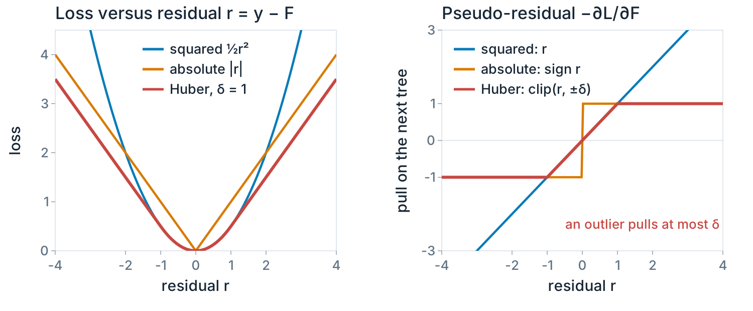
For MSE the residual is minus the gradient. For any differentiable loss define the pseudo-residual

$$r_{im}=-\left[\frac{\partial L(y_i,F)}{\partial F}\right]_{F=F_{m-1}(x_i)} .$$

Treat the $N$ values $F(x_1),\ldots,F(x_N)$ as parameters. $-\partial L/\partial F$ is the direction of steepest descent. The tree generalizes that direction to all $x$.

Gradient boosting = gradient descent in function space.

Loss $L(y,F)$	Pseudo-residual $r$
$\tfrac12(y-F)^2$	$y-F$
$\lvert y-F\rvert$	$\operatorname{sign}(y-F)$
Huber, width $\delta$	$y-F$, clipped to $[-\delta,\delta]$
BCE, $y\in\{0,1\}$	$y-\sigma(F)$

$\sigma(F)=1/(1+e^{-F})$ is defined on the classification slides.

Friedman’s recipe: fit a least-squares regression tree to the pseudo-residuals, then set each leaf value by the leaf-wise argmin of the true loss (a line search). The next slide replaces this line search with a second-order Taylor expansion, as in XGBoost, which also gives a split criterion for any loss.

Leaf values for any loss

Expand each event’s loss around the current prediction, to second order in the small update $\gamma$:

$$L\big(y_i,F_{m-1}(x_i)+\gamma\big)\approx L\big(y_i,F_{m-1}(x_i)\big)+g_i\,\gamma+\tfrac12 h_i\,\gamma^2, \qquad g_i=\frac{\partial L}{\partial F}\bigg|_{F_{m-1}(x_i)},\;\; h_i=\frac{\partial^2 L}{\partial F^2}\bigg|_{F_{m-1}(x_i)} .$$

In leaf $j$ sum the derivatives: $G_j=\sum_{i\in R_{mj}}g_i$, $\;H_j=\sum_{i\in R_{mj}}h_i$. Add a penalty $\tfrac12\lambda\gamma^2$ ($\lambda\ge0$) against large leaf values:

$$\text{leaf objective}\;=\;G_j\gamma+\tfrac12\big(H_j+\lambda\big)\gamma^2 \quad\xrightarrow{\;\partial/\partial\gamma=0\;}\quad \gamma_{mj}^{*}=-\frac{G_j}{H_j+\lambda}, \qquad\text{loss change}=-\frac12\,\frac{G_j^2}{H_j+\lambda}.$$

This is one Newton step per leaf. Check with MSE: $g_i=F-y_i=-r_i$, $h_i=1$, so $\gamma^*_{mj}=\sum r_i/(N_j+\lambda)$, the mean residual for $\lambda=0$.

T. Chen, C. Guestrin, “XGBoost: A Scalable Tree Boosting System”, KDD 2016, arXiv:1603.02754.

g is the gradient and h the curvature (Hessian) of the per-event loss with respect to the model output. For MSE the expansion is exact. Large curvature means a confident, well-determined leaf; small curvature allows a larger step. lambda shrinks leaf values toward zero, most strongly in leaves with small H.

Split gain for any loss

Insert the best leaf values into the objective. Splitting node $I$ into $I_L$ and $I_R$ reduces the loss by

$$\text{Gain}=\frac12\left[\frac{G_L^2}{H_L+\lambda}+\frac{G_R^2}{H_R+\lambda}-\frac{G_I^2}{H_I+\lambda}\right]-\tau ,$$

with $G_L=\sum_{i\in I_L}g_i$, $H_L=\sum_{i\in I_L}h_i$, and likewise for $I_R$ and the parent $I$.

Term	Meaning
$\dfrac{G^2}{H+\lambda}$	how much a node could lower the loss with its best single value
$\lambda\ge0$	leaf-value penalty: shrinks $\gamma^*$, disfavours leaves with little curvature $H$
$\tau\ge0$	cost of one extra leaf: split only if the improvement exceeds $\tau$ (gamma in XGBoost)

Same search as before: sort, scan cuts with running sums $G_L,H_L$, keep the best. For MSE with $\lambda=\tau=0$ this is the gain of the regression slide.

The original slide used the same letter gamma for the split cost and for the leaf values. Here the split cost is called tau to avoid the clash; XGBoost calls it gamma and calls leaf values w. With lambda = 0 and MSE, G = -sum r and H = N, so G^2/H = (sum r)^2 / N.

The general algorithm

1. $F_0=\arg\min_c\sum_i L(y_i,c)$.
2. For $m=1,\ldots,M$:
   1. compute $g_i$ and $h_i$ at $F_{m-1}(x_i)$ for every event;
   2. grow a tree: at each node choose the $(k,c)$ with the largest $\text{Gain}$; stop at the depth limit or if no gain is positive;
   3. leaf values $\gamma_{mj}=-G_j/(H_j+\lambda)$;
   4. update $F_m(x)=F_{m-1}(x)+\eta\sum_j\gamma_{mj}\mathbf 1[x\in R_{mj}]$.
3. Output $F_M(x)$, or $p(x)=\sigma\big(F_M(x)\big)$ for classification.

Only $g_i$ and $h_i$ depend on the loss.

Changing the task means changing two derivatives, not the tree code.

The trees in round $m$ never see the labels directly, only $g_i$ and $h_i$.

This is the loop implemented in widgets/gb.js (about 40 lines) and in the Pluto notebook. Newton mode uses h from the loss; gradient mode sets h_i = 1, which fits the pseudo-residuals by least squares and uses their mean as the leaf value.

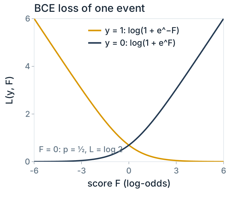
Classification: the score is a log-odds

Labels $y\in\{0,1\}$. Trees add up to an unbounded score $F(x)\in\mathbb R$; map it to a probability with the logistic function

$$p(x)=\sigma\big(F(x)\big)=\frac1{1+e^{-F(x)}},\qquad F=\log\frac{p}{1-p}.$$

Loss: binary cross-entropy (negative log-likelihood)

$$L(y,F)=-\big[y\log p+(1-y)\log(1-p)\big]$$ $$\phantom{L(y,F)}=\log\!\big(1+e^{F}\big)-yF .$$

The original slide showed the log-likelihood y F - log(1 + e^F), which is maximized; the loss is its negative. Boosting p directly would be awkward because a sum of trees can leave [0, 1]. A wrong but confident prediction is penalized roughly linearly in |F|, a correct one costs almost nothing.

BCE: gradients and leaf values

With $p_i=\sigma\big(F_{m-1}(x_i)\big)$, using $\frac{d\sigma}{dF}=\sigma(1-\sigma)$:

$$g_i=\frac{\partial L}{\partial F}=p_i-y_i,\qquad h_i=\frac{\partial^2 L}{\partial F^2}=p_i(1-p_i).$$

Pseudo-residual: $r_i=y_i-p_i$, the probability still missing.

Newton leaf value:

$$\gamma_{mj}=\frac{\sum_{i\in R_{mj}}(y_i-p_i)}{\sum_{i\in R_{mj}}p_i(1-p_i)+\lambda}.$$

Start: $F_0=\log\dfrac{\bar y}{1-\bar y}$, the log-odds of the signal fraction $\bar y$.

Worked example. Balanced sample, so $F_0=0$ and all $p_i=\tfrac12$. One leaf holds $y=1,1,1,0$:

• $g=-\tfrac12,-\tfrac12,-\tfrac12,+\tfrac12\Rightarrow G=-1$
• $h=\tfrac14$ each $\Rightarrow H=1$
• $\lambda=0$: $\gamma=1$ (leaf log-odds $\log3=1.10$)
• $\eta=0.3$: $F=0.3$, $p=\sigma(0.3)=0.57$

Derivation: d/dF log(1+e^F) = e^F/(1+eF) = p, so g = p - y; h = dp/dF = p(1-p). One Newton step lands close to the leaf’s own log-odds. With gradient-mode leaves (h = 1) the same leaf would get gamma = mean(y - p) = 0.25, a much smaller step. Near-pure leaves have tiny H; lambda (and XGBoost’s min_child_weight, a minimum H) keeps their values finite.

One algorithm, two losses

	Regression: MSE	Classification: BCE
Label and output	$y\in\mathbb R$, prediction $F$	$y\in\{0,1\}$, log-odds $F$, $p=\sigma(F)$
Loss $L(y,F)$	$\tfrac12(y-F)^2$	$\log(1+e^{F})-yF$
Start $F_0$	$\bar y$	$\log\big(\bar y/(1-\bar y)\big)$
Gradient $g_i$	$F_{m-1}(x_i)-y_i$	$p_i-y_i$
Curvature $h_i$	$1$	$p_i(1-p_i)$
Leaf value $\gamma_{mj}$	$\dfrac{\sum(y_i-F_{m-1}(x_i))}{N_j+\lambda}$	$\dfrac{\sum(y_i-p_i)}{\sum p_i(1-p_i)+\lambda}$
Split gain	$\tfrac12\big[G_L^2/(H_L{+}\lambda)+G_R^2/(H_R{+}\lambda)-G_I^2/(H_I{+}\lambda)\big]-\tau$	same formula
Prediction	$F_M(x)$	$p(x)=\sigma\big(F_M(x)\big)$, cut on $p$

The summary slide students should be able to reconstruct. Sums in the leaf-value row run over events in leaf j. The classifier output is a probability-like score; choose the working point on p with the ROC curve from Lecture 2A.

Boosting a classifier

Widget 3. Left: p(x) after m trees; point area is |y - p|, the pseudo-residual magnitude, so points that are already well classified shrink. Middle: the contribution eta * gamma_m(x) of the current tree, drawn over the residuals it was fitted to; gold regions push toward signal, blue toward background. Right: mean BCE on training and validation samples. Suggestions: step through m = 1..5 on the disk; switch to xor with depth 1 (stumps cannot find a first useful cut, since each single cut has zero expected gain) then depth 2; compare Newton and gradient leaves; set eta = 1, depth 4 and watch the validation BCE rise. Leaf penalty lambda = 1 throughout. Labels have 6% random flips.

Regularization

A boosted ensemble can always lower its training loss. These controls keep the validation loss low:

Control	Effect
Shrinkage $\eta$	small steps; smaller $\eta$ needs more trees $M$ but usually generalizes better
Tree depth (1–5 typical)	depth $D$ allows interactions among up to $D$ features; shallow trees are weak learners
Subsampling	each tree sees a random fraction of events (stochastic gradient boosting)
Leaf penalties $\lambda$, $\tau$, minimum $H$ per leaf	limit leaf values and forbid tiny or uninformative leaves
Early stopping	stop at the $M$ with the lowest validation loss

Friedman (2002) introduced stochastic gradient boosting with subsampling fraction around 0.5 to 0.8. Early stopping requires a validation sample that is not the final test sample. Shrinkage and number of trees trade off: roughly, eta times M sets how far the model can move.

Huber loss: robust regression

With $r=y-F$ and a width $\delta>0$:

$$L_\delta(r)=\begin{cases}\tfrac12r^2, & |r|\le\delta,\\[2pt] \delta\big(|r|-\tfrac12\delta\big), & |r|>\delta.\end{cases}$$

• Quadratic near 0: as efficient as least squares for Gaussian errors.
• Linear in the tails: robust like absolute loss.
• Pseudo-residual: $r$ clipped to $[-\delta,\delta]$. An outlier’s pull is capped.

Friedman chooses delta adaptively as a quantile (e.g. 90%) of the current absolute residuals. For |r| > delta the second derivative is zero, so Newton leaves need care; Friedman uses a robust leaf estimate (median plus a clipped mean correction).

Other losses for classification

Binomial deviance, $y\in\{-1,+1\}$

$$L(y,F)=\log\big(1+e^{-2yF}\big),\qquad r=-\frac{\partial L}{\partial F}=\frac{2y}{1+e^{2yF}} .$$

Friedman’s convention. It is the BCE of the previous slides with labels $\tfrac{1+y}{2}\in\{0,1\}$ and score $2F$, so $F=\tfrac12\log\frac p{1-p}$.

Exponential loss, $y\in\{-1,+1\}$

$$L(y,F)=e^{-yF},\qquad g_i=-y_i\,e^{-y_iF(x_i)} .$$

The factor $e^{-y_iF(x_i)}$ is exactly the AdaBoost event weight: boosting with this loss reproduces AdaBoost.

It grows exponentially for badly misclassified events, hence the noise sensitivity.

Friedman, Hastie, Tibshirani, “Additive logistic regression: a statistical view of boosting”, Ann. Stat. 28 (2000) 337. The derivative of log(1+e^{-2yF}) is -2y e^{-2yF}/(1+e{-2yF}) = -2y/(1+e^{2yF}); the pseudo-residual is its negative. Compare the losses at large negative margin yF: deviance grows linearly, exponential loss exponentially.

Libraries and their parameter names

Symbol	XGBoost	ROOT TMVA (BDT)
$M$	n_estimators	NTrees
$\eta$	learning_rate (eta)	Shrinkage
depth	max_depth	MaxDepth
subsample	subsample	BaggedSampleFraction
$\lambda$	reg_lambda	—
$\tau$	gamma	—
loss	objective	BoostType=Grad

Also: LightGBM, CatBoost; in Julia XGBoost.jl, EvoTrees.jl, JLBoost.jl.

import xgboost as xgb
clf = xgb.XGBClassifier(
    objective="binary:logistic",  # BCE
    n_estimators=500, learning_rate=0.1,
    max_depth=3, reg_lambda=1.0,
    subsample=0.8, early_stopping_rounds=20)
clf.fit(X_train, y_train,
        eval_set=[(X_val, y_val)])
p = clf.predict_proba(X_test)[:, 1]

Regression: XGBRegressor with
objective="reg:squarederror".

XGBoost (C++) has Python, R and Julia interfaces. TMVA’s BDT also offers AdaBoost and bagging via BoostType; UseBaggedBoost enables subsampling. TMVA users guide: https://root.cern.ch/download/doc/tmva/TMVAUsersGuide.pdf. Early stopping monitors the last entry of eval_set.

Impact of boosted trees

• State of the art on tabular data. Of 29 winning Kaggle solutions published in 2015, 17 used XGBoost; 8 used it alone.
• Industry: risk modelling in finance, click-through-rate prediction, insurance, customer modelling. Accurate, fast, and comparatively interpretable.
• High-energy physics: for years the most common architecture for signal/background separation at the LHC, e.g. in the Higgs discoveries and flavour tagging.

Kaggle statistic: Chen & Guestrin, arXiv:1603.02754.

Boosted decision trees remain strong baselines for tabular data even where neural networks are used, and are often combined with them in ensembles.

BDT playground

Online: Alex Rogozhnikov’s gradient boosting playground and explanation.

Julia: a Pluto adaptation with JLBoost.jl: static preview · source

Live version, from this lecture’s folder:

julia notebooks/launch.jl

Tasks

1. Reach a test loss below 0.05 on every dataset.
2. Which datasets need depth $\ge2$? Why?
3. Fix $\eta M$ and compare $\eta=1$ with $\eta=0.1$.
4. Compare Newton and gradient updates at equal $M$.

The Pluto notebook offers six datasets, rotations, depth, learning rate, subsampling, Newton/gradient updates, and per-tree contribution maps. The static preview needs Pluto’s CDN; live controls need the launcher.

End

Thank you for the attention