Decision Trees

Mikhail Mikhasenko · Lecture 2A

Decision trees

A sequence of simple questions partitions feature space.

  • At each node, choose a feature and a cut.
  • Send each event to the left or right child.
  • A leaf returns a class, a class fraction, or a regression value.
f1<c1f_1 < c_1?
yes
f2<c2f_2 < c_2?
signalbackground
no
f2<c3f_2 < c_3?
backgroundsignal

Reminder: cutting distributions

For a selection x<cx<c:

ϵS=SpassSall,rB=1−BpassBall\epsilon_S=\frac{S_{\mathrm{pass}}}{S_{\mathrm{all}}},\qquad r_B=1-\frac{B_{\mathrm{pass}}}{B_{\mathrm{all}}}

p=SpassSpass+Bpassp=\frac{S_{\mathrm{pass}}}{S_{\mathrm{pass}}+B_{\mathrm{pass}}}

Efficiency and purity answer different questions.

The ROC curve traces the operating points as the threshold moves.

Here the vertical axis is background rejection, 1−ϵB1-\epsilon_B.

Purity also depends on the signal fraction before selection.

One cut, three competing goals

Splitting index

A useful cut depends on the objective.

Objective Example What it measures
Select a sample Purity S/(S+B)S/(S+B) Composition after selection
Retain signal Efficiency S/SallS/S_{\mathrm{all}} Signal survival
Estimate sensitivity S/S+BS/\sqrt{S+B} A simple counting proxy
Grow a tree Gini or entropy gain Improvement in both children

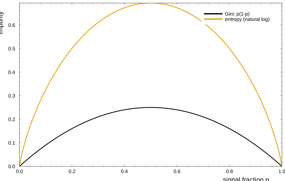
Gini impurity

If pp is the weighted signal fraction,

p=∑i∈Swi∑iwi,IG=p(1−p).p=\frac{\sum_{i\in S}w_i}{\sum_i w_i},\qquad I_G=p(1-p).

A pure node has IG=0I_G=0. A balanced node has IG=1/4I_G=1/4.

The standard binary Gini impurity is 2p(1−p)2p(1-p). The factor of two does not change the best split.

Gini and entropy as functions of class fraction

Making a single split

1. Unweighted events 2. Weighted events
For node RR, use event counts:

NR=|R|,pR=NS,RNR\displaystyle N_R=|R|,\quad p_R=\frac{N_{S,R}}{N_R}
Replace counts by sums of weights:

WR=∑i∈Rwi,pR=∑i∈R,yi=1wiWR\displaystyle W_R=\sum_{i\in R}w_i,\quad p_R=\frac{\sum_{i\in R,\,y_i=1}w_i}{W_R}
Score the cut with total impurity decrease:

G=N0I(p0)−NLI(pL)−NRI(pR)\displaystyle G=N_0I(p_0)-N_LI(p_L)-N_RI(p_R)
Use the normalized weighted decrease:

ΔI=I(p0)−WLW0I(pL)−WRW0I(pR)\displaystyle \Delta I=I(p_0)-\frac{W_L}{W_0}I(p_L)-\frac{W_R}{W_0}I(p_R)

Search all allowed features and thresholds, then choose the largest positive gain. Multiplying ΔI\Delta I by W0W_0 recovers GG.

Where should the tree split?

Growing a tree

Sampling model used here

The two features are independent:

X1,X2∼iidUniform(0,1).X_1,X_2\overset{\mathrm{iid}}{\sim}\operatorname{Uniform}(0,1).

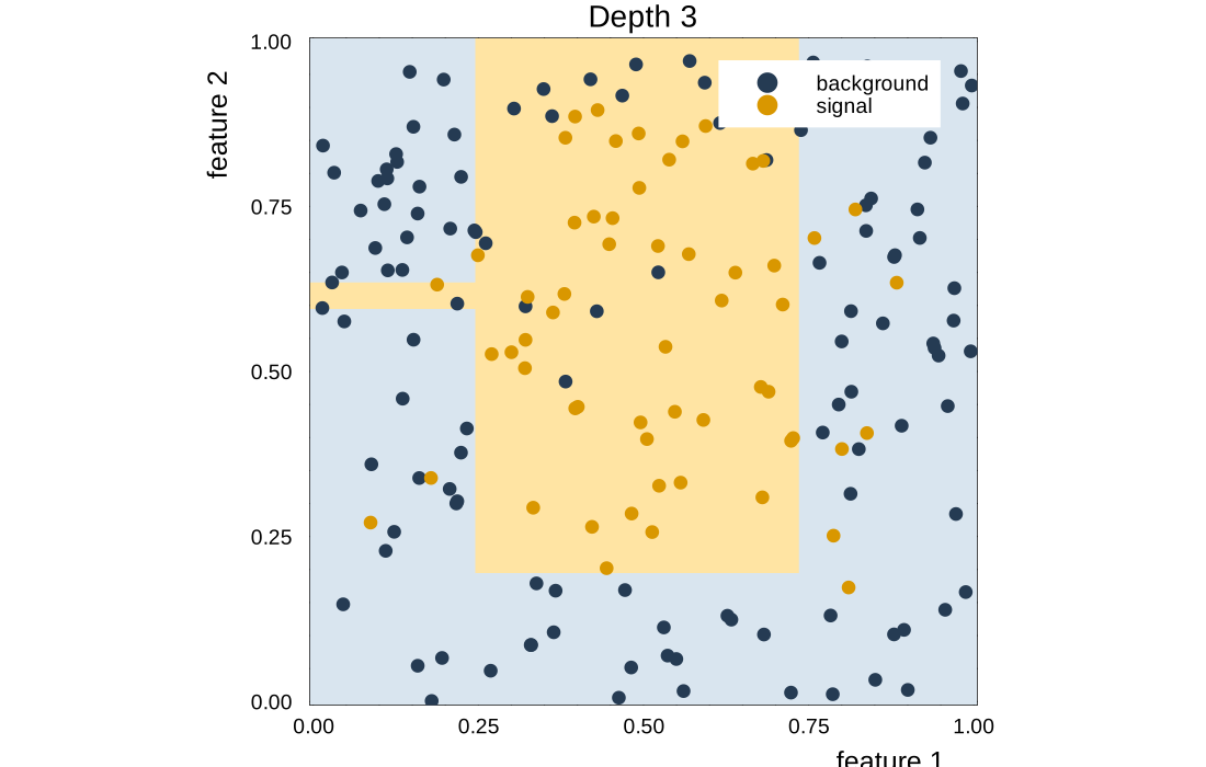
The noiseless label is signal inside an ellipse:

y*=+1⇔(X1−0.50)20.075+(X2−0.55)20.13<1.y^*=+1\iff \frac{(X_1-0.50)^2}{0.075}+\frac{(X_2-0.55)^2}{0.13}<1.

Each label flips independently with probability 0.080.08. The training sample contains N=180N=180 events generated with seed 21.

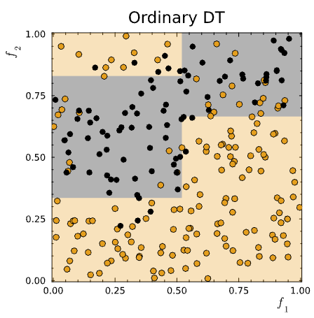
Julia-trained depth-three tree and its axis-aligned decision regions

Both features are searched at every node. Candidate cuts are midpoints between consecutive observed values; leaves contain at least two events.

How well does it do?

accuracy=NcorrectNevents\mathrm{accuracy}=\frac{N_{\mathrm{correct}}}{N_{\mathrm{events}}}

Training: fit the splits and leaf predictions.

Validation: choose depth and other settings.

Test: assess the chosen model once.

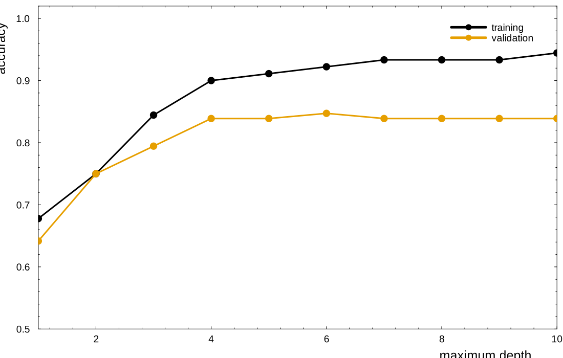
A model can improve on training data while getting worse on new data.

Keep the data split fixed while comparing settings.

For imbalanced classes, inspect class efficiencies and ROC curves as well as accuracy.

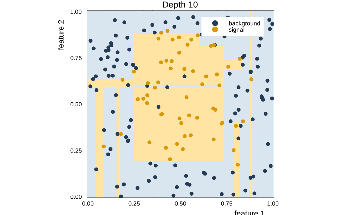
Overtraining

A deeper tree introduces small regions around noisy training events

Training and validation accuracy versus maximum tree depth, calculated in Julia

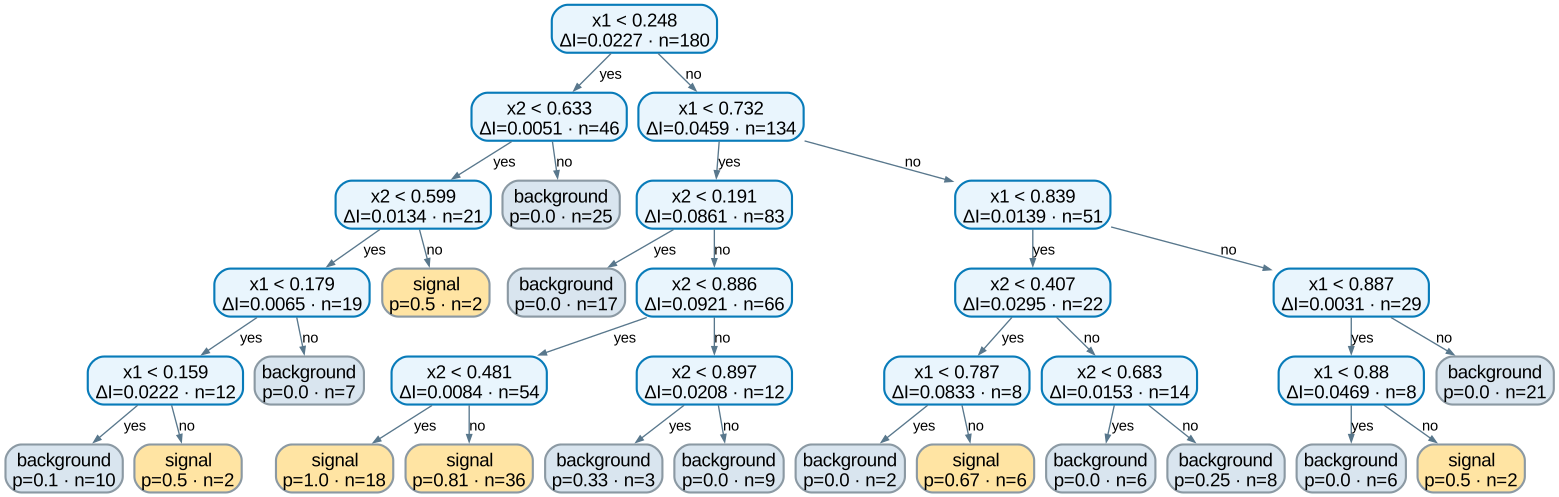
A fitted tree at depth 5

Complete fitted depth-five decision tree showing the feature and threshold at each split and the class probability at every leaf

Each internal node shows the selected feature, cut, and impurity gain. Each leaf shows its prediction, signal fraction pp, and number of training events nn.

Bagging as random event reweighting

Start from D={(xi,yi)}i=1ND=\{(x_i,y_i)\}_{i=1}^{N}. For tree bb, draw NN indices with replacement. The multiplicities obey

(K1(b),…,KN(b))∼Multinomial(N;1N,…,1N). (K_1^{(b)},\ldots,K_N^{(b)}) \sim\operatorname{Multinomial}\!\left(N;\frac1N,\ldots,\frac1N\right).

The bootstrap sample is the original sample with random integer weights

wi(b)=Ki(b),WR(b)=∑i∈RKi(b).w_i^{(b)}=K_i^{(b)},\qquad W_R^{(b)}=\sum_{i\in R}K_i^{(b)}.

Mean multiplicity Omitted events Repeated events
𝔼[Ki(b)]=1\mathbb E[K_i^{(b)}]=1 P(Ki(b)=0)=(1−1/N)N≈e−1P(K_i^{(b)}=0)=(1-1/N)^N\approx e^{-1} P(Ki(b)≥2)≈1−2e−1P(K_i^{(b)}\ge2)\approx1-2e^{-1}
Average weight is unchanged About 63.2%63.2\% appear at least once About 26.4%26.4\% appear more than once

Combining the bagged trees

Tree bb sends a new event xx to a leaf Lb(x)L_b(x). Its signal probability is the weighted signal fraction in that leaf:

p̂b(x)=∑i:xi∈Lb(x)Ki(b)yi∑i:xi∈Lb(x)Ki(b). \hat p_b(x)= \frac{\sum_{i:\,x_i\in L_b(x)}K_i^{(b)}y_i} {\sum_{i:\,x_i\in L_b(x)}K_i^{(b)}}.

Ordinary bagging gives every trained tree the same prediction weight:

p̂bag(x)=1B∑b=1Bp̂b(x),ŷbag(x)=𝟏[p̂bag(x)>12]. \hat p_{\mathrm{bag}}(x)=\frac1B\sum_{b=1}^{B}\hat p_b(x), \qquad \hat y_{\mathrm{bag}}(x)=\mathbf 1\!\left[\hat p_{\mathrm{bag}}(x)>\tfrac12\right].

For hard tree labels ŷb(x)∈{0,1}\hat y_b(x)\in\{0,1\}, majority voting uses 𝟏[∑bŷb(x)>B/2]\mathbf 1[\sum_b\hat y_b(x)>B/2]. For regression, average the numerical tree predictions.

Options for a bagged tree ensemble

Useful ensembles reduce shared errors between trees while controlling how each tree grows.

What changes for tree bb? Construction Common name
Training events Draw events with replacement, or use a random subsample Bagging
Available features At each node, search only mtry<pm_{\mathrm{try}}<p randomly selected features Random forest
Candidate cuts Test random thresholds instead of every possible threshold Extremely randomized trees
Growth rule Control maximum depth, minimum leaf size, or pruning Regularized trees

Removing features temporarily can force trees to discover alternative predictors. The aim is to reduce correlation ρ\rho between trees while keeping each tree useful:

Var(1B∑b=1Bhb)≈σ2[ρ+1−ρB]. \operatorname{Var}\!\left(\frac1B\sum_{b=1}^{B}h_b\right) \approx \sigma^2\!\left[\rho+\frac{1-\rho}{B}\right].

Depth and bagging

Bagging

Bootstrap aggregating

  1. Draw a training sample with replacement.
  2. Train a tree on that sample.
  3. Repeat, then average predictions or vote.

Different samples produce different trees. Averaging can reduce variance.
Example ensemble settings:

n_trees = 30
max_depth = 6
partial_sampling = 0.7
n_subfeatures = 2

A random forest also samples the candidate features at each split. Using both of two features adds no feature randomness.

Julia: regression trees

The same partitioning idea works for continuous targets.

Each leaf predicts its training mean:

ŷR=1NR∑i∈Ryi.\hat y_R=\frac{1}{N_R}\sum_{i\in R}y_i.

Squared-error splits prefer regions with less target variation.

using DecisionTree
X = reshape(x_train, :, 1)
model = DecisionTreeRegressor(
    max_depth=5, rng=123)
fit!(model, X, y_train)
yhat = predict(model, X_validation)

Open the regression notebook · Julia source

Julia notebooks

Notebook Experiment Lecture connection
Cuts and impurity Move the cut and vary the mixture ROC, purity, split gain
Classification trees Change depth, tree count, boosting rounds Boundaries, overtraining, ensembles
Regression trees Fit 1D and 2D functions Piecewise predictions, forests, losses

The slide figures and widget models come from the same seeded Julia calculations.

Boosting

AdaBoost trains weak classifiers in sequence.

  1. Start with equal event weights.
  2. Fit a classifier using the current weights.
  3. Increase the relative weight of mistakes.
  4. Add the classifier to a weighted vote.

Bagging: different resampled datasets, independently trained trees.

Boosting: each fit depends on earlier mistakes.

A weak learner needs an error below 1/21/2 in the binary setting.

AdaBoost: weights and votes

For labels and predictions yi,hm(xi)∈{−1,+1}y_i,h_m(x_i)\in\{-1,+1\}:

ϵm=∑iwi(m)𝟏[hm(xi)≠yi]∑iwi(m),αm=12log1−ϵmϵm\epsilon_m=\frac{\sum_i w_i^{(m)}\,\mathbf{1}[h_m(x_i)\ne y_i]}{\sum_i w_i^{(m)}}, \qquad \alpha_m=\frac12\log\frac{1-\epsilon_m}{\epsilon_m}

wi(m+1)∝wi(m)e−αmyihm(xi),H(x)=sign(∑m=1Mαmhm(x))w_i^{(m+1)}\propto w_i^{(m)}e^{-\alpha_m y_i h_m(x_i)}, \qquad H(x)=\operatorname{sign}\!\left(\sum_{m=1}^M\alpha_m h_m(x)\right)

Normalize the event weights after each round.

AdaBoost pays attention to mistakes

Original sample

Two measured features, overlapping classes.

A tree approximates the separating boundary with axis-aligned regions.

Noise and class overlap limit what any fitted boundary can achieve.

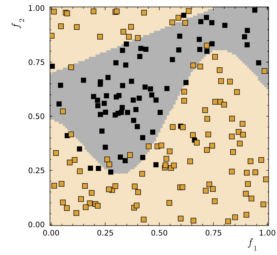
Original lecture's two-feature signal and background sample

Quiz

Looking at this classification, draw a possible tree.

  • Which feature could the first split use?
  • Which later cuts apply only inside one region?
  • Can different trees produce the same partition?

Original decision-tree partition for students to reconstruct

End

Thank you for the attention