Key notions in ML

Introduction

Mikhail Mikhasenko, 29/07/2025

Plan for the course

AD

Decision
Tree

Dense
Nets

Transformers

ML

Supervised learning

Labelled data

Machine-learning language:

  • xx is a feature vector, x=(xf1,xf2,…,xfN)x=(x^{f_1},x^{f_2},\ldots,x^{f_N})
  • yy is a label: a value, a vector, or a class such as cat/dog or signal/background
  • The data are pairs: {(xi,yi)}i=1n\{(x_i,y_i)\}_{i=1}^{n}

f(x)=yf(x)=y

we want to learn

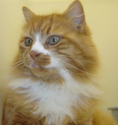
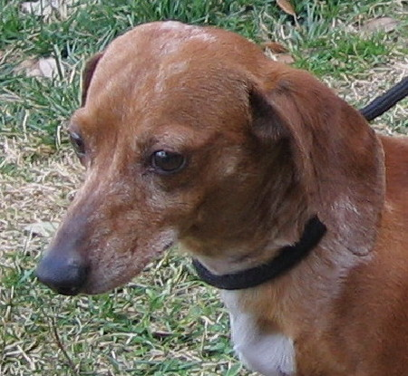
Regression and classification

  • Classification: yy belongs to a discrete set of classes
  • Regression: yy belongs to a continuous space

f(x)=yf(x)=y

Labels and features

Kaggle and ML datasets

  • Large collection of datasets and machine-learning challenges
  • Public notebooks, benchmarks, and competitions

Kaggle home page advertising its datasets and ML community

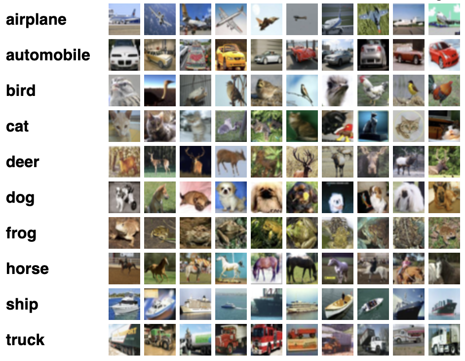
Example 1: Image classification

  • Problem: recognize the object in an image
  • Label: class name

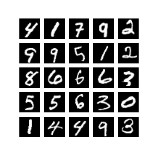
Example 1: one MNIST image

A handwritten seven drawn as a grayscale image

One training example is a 28 × 28 image: 784 grayscale pixel values.

The label is a single digit. MNIST has 10 classes, the digits 0 through 9.

MNIST

Example 1: input and output

Input

Handwritten seven used as the model input

784 pixel values

ML

Output

0

1

2

3

4

5

6

7

8

9

10 class scores

Example 2: Predicting housing prices

  • Problem: predict a house price from its features
  • Feature space: rooms, location, area, condition, and similar descriptors
  • Label: a real-valued price

Kaggle House Prices competition

Rows of houses with different roof and building features

Example 2: the data fields

79 data fields in, one price out

MSSubClass · MSZoning · LotFrontage · LotArea · Street · Alley · LotShape · LandContour · Utilities · LotConfig · LandSlope · Neighborhood · Condition1 · Condition2 · BldgType · HouseStyle · OverallQual · OverallCond · YearBuilt · YearRemodAdd · RoofStyle · RoofMatl · Exterior1st · Exterior2nd · MasVnrType · MasVnrArea · ExterQual · ExterCond · Foundation · BsmtQual · BsmtCond · BsmtExposure · BsmtFinType1 · BsmtFinSF1 · BsmtFinType2 · BsmtFinSF2 · BsmtUnfSF · TotalBsmtSF · Heating · HeatingQC · CentralAir · Electrical · 1stFlrSF · 2ndFlrSF · LowQualFinSF · GrLivArea · BsmtFullBath · BsmtHalfBath · FullBath · HalfBath · BedroomAbvGr · KitchenAbvGr · KitchenQual · TotRmsAbvGrd · Functional · Fireplaces · FireplaceQu · GarageType · GarageYrBlt · GarageFinish · GarageCars · GarageArea · GarageQual · GarageCond · PavedDrive · WoodDeckSF · OpenPorchSF · EnclosedPorch · 3SsnPorch · ScreenPorch · PoolArea · PoolQC · Fence · MiscFeature · MiscVal · MoSold · YrSold · SaleType · SaleCondition

Id is only an index. SalePrice is the label, not a feature. Competition data

Example 2: input and output

Input · 79 fields
LotArealot size, square feet 8450
OverallQualmaterial and finish, 1–10 7
YearBuiltyear of construction 2003
GrLivAreaabove-ground living area, square feet 1710
GarageCarsgarage capacity, in cars 2
and 74 further fields

ML

Output
$208,500
SalePrice

Example 3: Balancing a pole

  • Problem: keep a pole upright by moving a cart left or right
  • Feature space: cart position and velocity, pole angle and angular velocity
  • Label: push left or push right
  • Setting: reinforcement learning

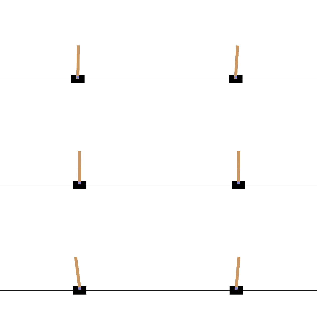
Gymnasium Cart Pole

Animated cart pole balancing a pole by moving the cart

Example 3: input and output

Input
Cart position 0.036
Cart velocity −0.089
Pole angle −0.056
Pole angular velocity −0.063

ML

Output

0 · push left

1 · push right

Learning the function

  • A mathematical algorithm adjusts ff so that f(x)f(x) predicts yy well on the data
  • Learning resembles adaptation in a biological brain: many parameters change, even when their individual meaning remains obscure

f(x)=yf(x)=y

Stylized neural network with inputs x and outputs y

Loss function

or score function

Glass illustrated as half empty and half full

Loss function

  • The loss quantifies how well the learned function f(x)f(x) describes the data
  • Training searches parameter space for a small loss
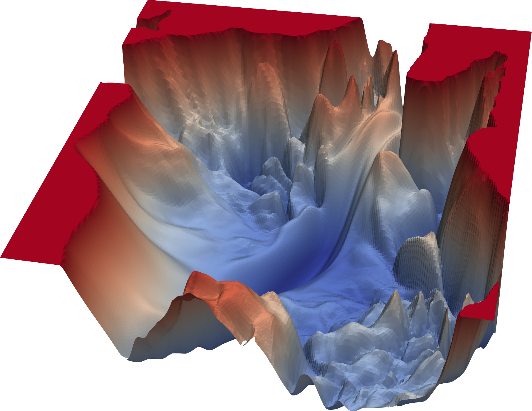
Complex loss landscape over two model parameters

Complex loss landscape as a function of parameters p̃1\tilde p_1 and p̃2\tilde p_2

Loss: Mean squared error

Hypothetical flat prices
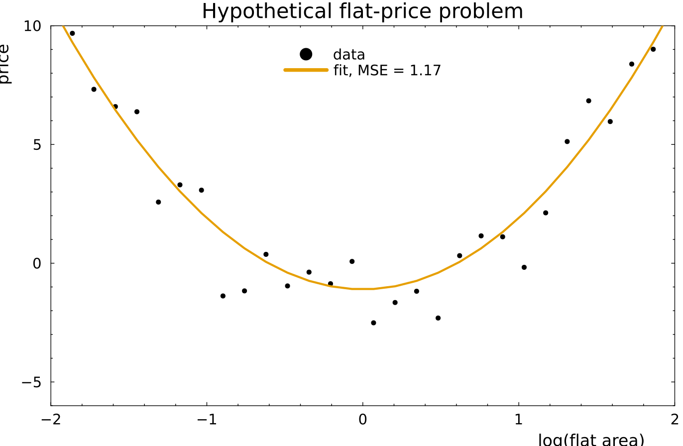
Quadratic price curve fitted to noisy flat-area data, with MSE 1.17

f(x)=3x2−a,a=1.1 f(x)=3x^2-a,\qquad a=1.1

MSE=1n∑i=1n(yi−f(xi))2=1.17 \operatorname{MSE}=\frac{1}{n}\sum_{i=1}^{n}\left(y_i-f(x_i)\right)^2=1.17

Thirty noisy prices. The curve is one setting of aa; training moves aa to make this loss small.

Reinforcement learning loss

General policy-gradient loss

L(θ)=−1N∑i=1N∑t=0Ti−1Gi,tlogπθ(ai,t∣si,t) L(\theta)=-\frac{1}{N}\sum_{i=1}^{N}\sum_{t=0}^{T_i-1} G_{i,t}\log \pi_\theta(a_{i,t}\mid s_{i,t})

Gi,t=∑k=tTi−1γk−tri,k G_{i,t}=\sum_{k=t}^{T_i-1}\gamma^{k-t}r_{i,k}

LL loss minimized in training
θ\theta neural-network parameters
NN episodes; ii episode index
TiT_i number of frames in episode ii
tt current frame; kk future frame
si,ts_{i,t} state; ai,ta_{i,t} chosen action
ri,kr_{i,k} reward; γ\gamma discount factor
Gi,tG_{i,t} future reward after the action
πθ(a∣s)\pi_\theta(a\mid s) action probability from the network
CartPole: the pole stays up for 120 frames

Every frame gives rt=1r_t=1. Choose γ=1\gamma=1.

Gt=∑k=t1191=120−t G_t=\sum_{k=t}^{119}1=120-t

Let pt=P(right∣st)p_t=P(\text{right}\mid s_t) and define the probability of the action taken:

qt={pt,at=right,1−pt,at=left. q_t=\begin{cases} p_t,& a_t=\text{right},\\ 1-p_t,& a_t=\text{left}. \end{cases}

Lepisode=−∑t=0119(120−t)logqt \boxed{L_{\mathrm{episode}}=-\sum_{t=0}^{119}(120-t)\log q_t}

Minimizing this loss makes actions from the observed 120-frame episode more probable.

Loss: Binary cross entropy

Standard for binary classification

  • Mean squared error can classify, but binary cross entropy better matches a probabilistic classifier
  • Interpret p(x)=f(x)p(x)=f(x) as the probability of class y=1y=1
  • The probability of class y=0y=0 is 1−p(x)1-p(x)

BCE=−∑i[yilogp(xi)+(1−yi)log(1−p(xi))] \operatorname{BCE}=-\sum_i\left[y_i\log p(x_i)+(1-y_i)\log\big(1-p(x_i)\big)\right]

The loss grows rapidly when the model assigns low probability to the observed class.

Shannon entropy

How broad, and how uncertain, a distribution is

S=−∑iqilogqi S=-\sum_i q_i\log q_i

S=−∫q(x)logq(x)dx S=-\int q(x)\log q(x)\,dx

Monte Carlo, with xix_i drawn from qq:

S≈−1n∑ilogq(xi) S\approx-\frac{1}{n}\sum_i\log q(x_i)

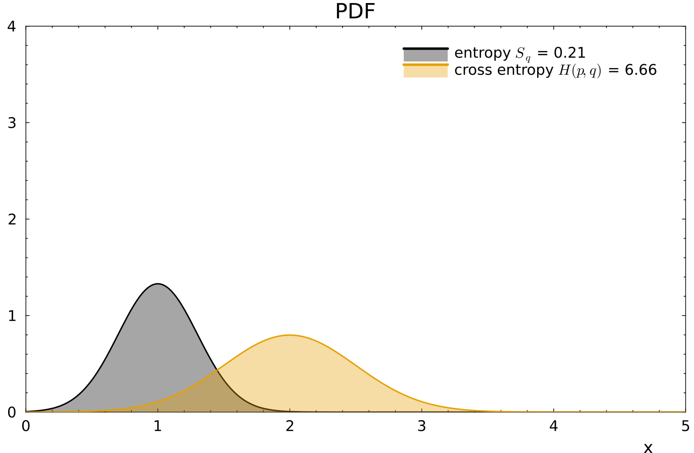
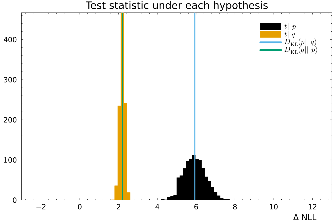
The narrow density has Sq=0.21S_q=0.21. A broader density is more uncertain, so its entropy is larger.

Cross entropy of two distributions

Likelihood of qq, evaluated on a sample from pp

H(p,q)=−∑ipilogqi H(p,q)=-\sum_i p_i\log q_i

  • This is binary cross entropy for two densities
  • It measures how different pp and qq are
  • The minimum is p=qp=q, and then H(p,p)H(p,p) is the entropy of pp

Narrow density q and broader reference p, with entropy 0.21 and cross entropy 6.66

q=Normal(1,0.3)q=\mathrm{Normal}(1,0.3), p=Normal(2,0.5)p=\mathrm{Normal}(2,0.5)

H(p,q)=6.66H(p,q)=6.66

Relative entropy

Kullback–Leibler divergence

DKL(p∥q)=H(p,q)−Sp D_{\mathrm{KL}}(p\|q)=H(p,q)-S_p

DKL(p∥q)=−∑ipilogqipi D_{\mathrm{KL}}(p\|q)=-\sum_i p_i\log\frac{q_i}{p_i}

Expected likelihood difference when the truth is pp and the model is qq. The two directions are not equal.

Sampled test statistic under each hypothesis, with both KL divergences marked

DKL(p∥q)=5.93D_{\mathrm{KL}}(p\|q)=5.93, DKL(q∥p)=2.19D_{\mathrm{KL}}(q\|p)=2.19

Training ML system

Training, validation, and test data

Minimal setup
  • Train on the training set
  • Evaluate once on the test set
Comparing architectures
  • Use a validation set for model and hyperparameter choices
  • Keep the test set independent until the final evaluation
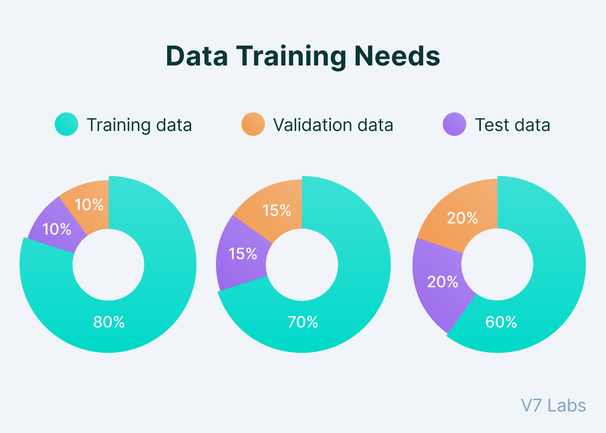
Example training, validation, and test splits

Classification decisions

  • A classifier usually returns a continuous score or probability
  • A threshold converts the score into a class decision
  • The error rate depends on the chosen threshold
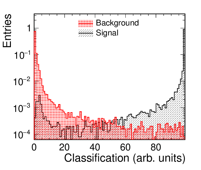
Signal and background classifier-score distributions

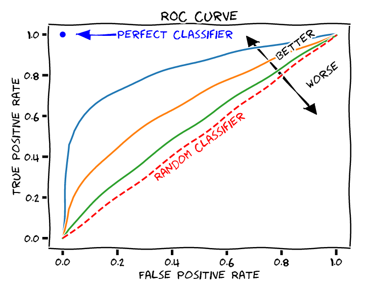
ROC curve

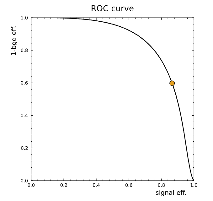
Receiver operating characteristic

  • Sweep the classifier threshold
  • Plot the true-positive rate against the false-positive rate
  • Curves closer to the upper-left corner indicate stronger separation
  • AUC, the area under the curve, summarizes the whole ROC: 11 is perfect, 12\tfrac12 is chance

Efficiency as a function of signal retained for one classifier threshold

The same threshold sweep in different variables
Illustrated ROC curves comparing perfect, better, random, and worse classifiers

Optimization and gradient descent

Training minimizes a loss L(θ)L(\theta) over model parameters θ\theta.

θt+1=θt−η∇θL(θt) \theta_{t+1}=\theta_t-\eta\,\nabla_{\theta}L(\theta_t)

  • Learning rate η\eta: the size of each step along the gradient
  • The gradient points toward the steepest local increase, so the update moves in the opposite direction

Complex loss landscape used to illustrate gradient-based optimization