Mikhail Mikhasenko
Why automatic differentiation?
From early neural networks to the need for reliable derivatives
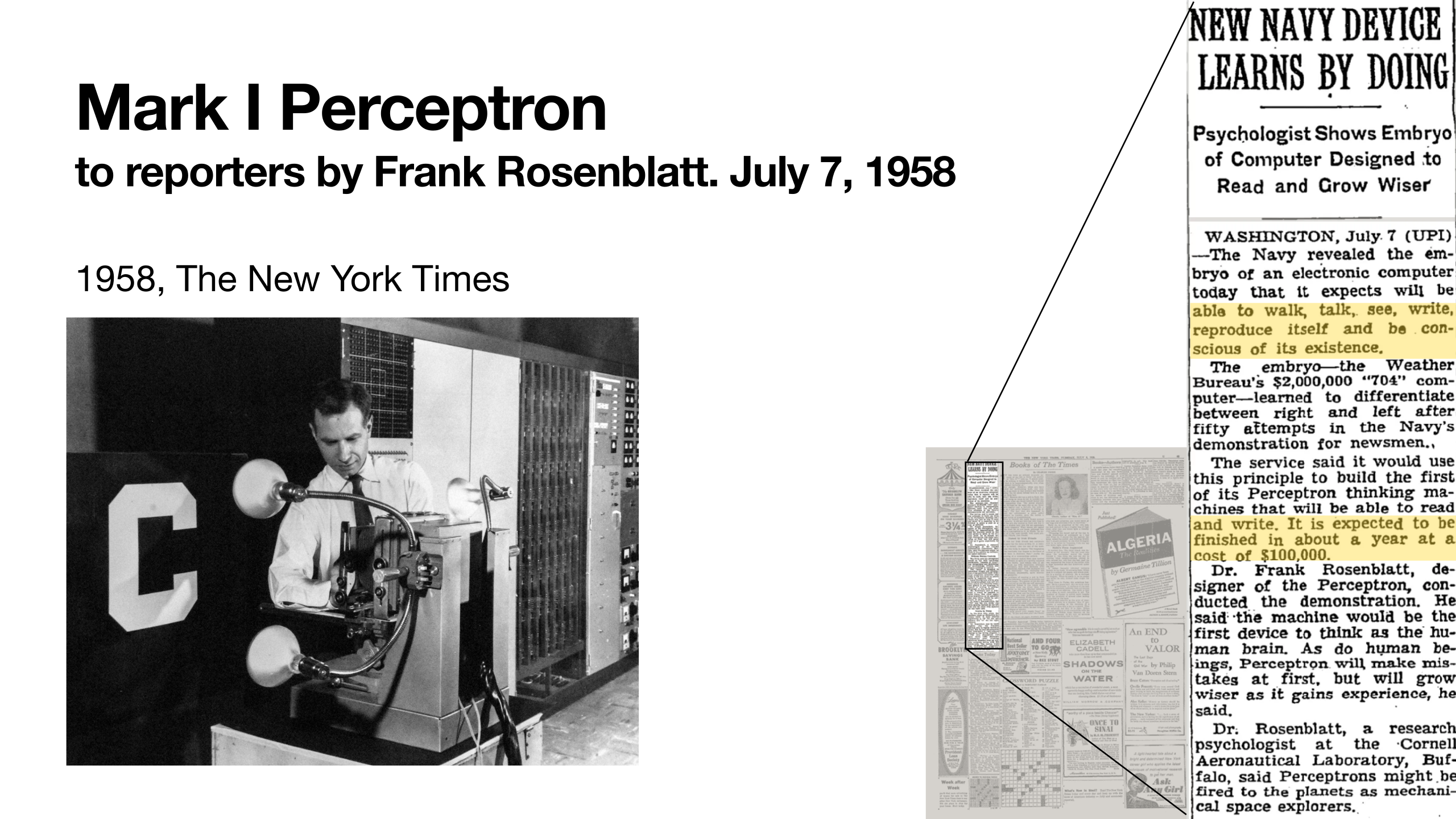
Mark I Perceptron
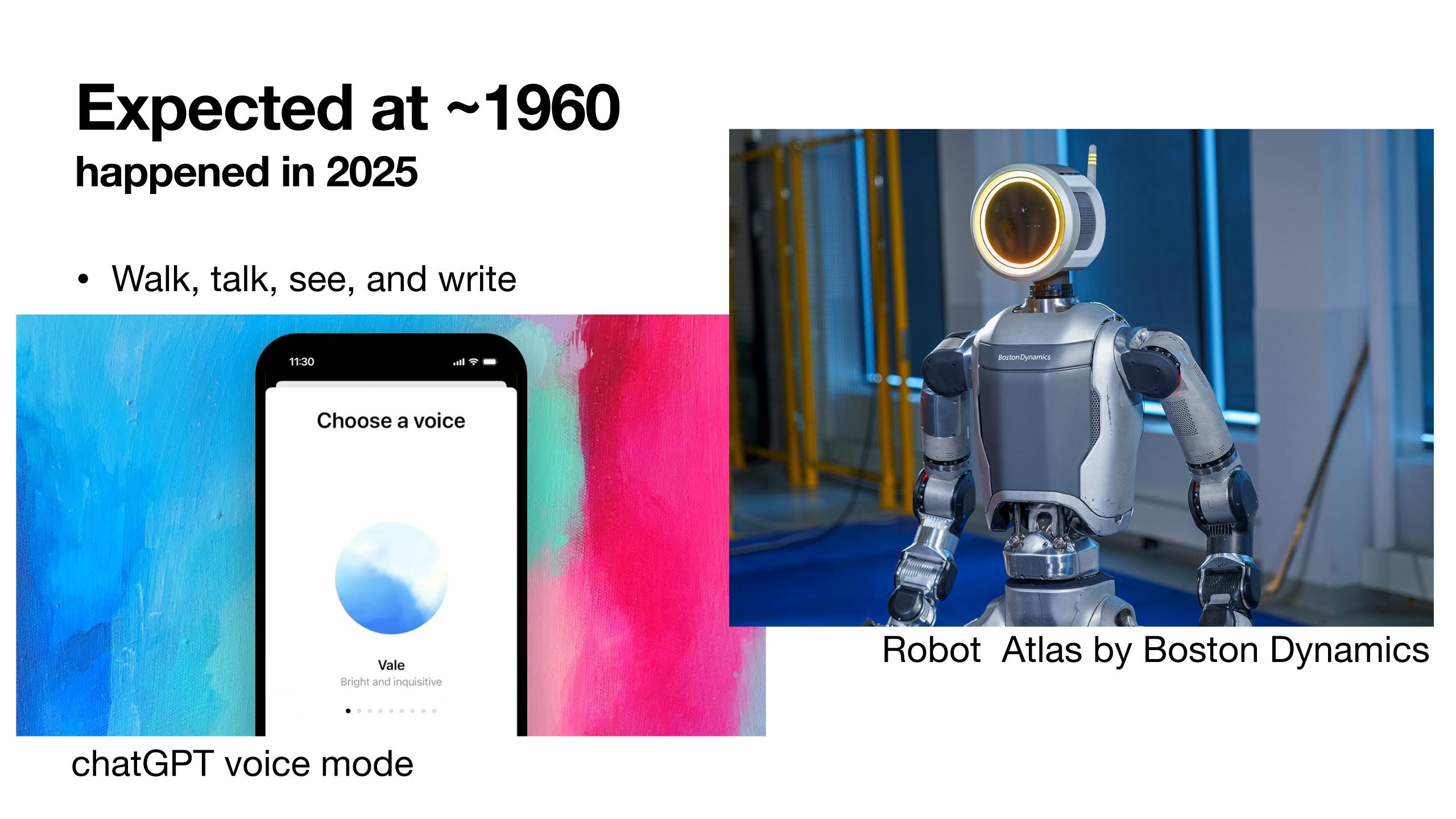
Expected at ~1960
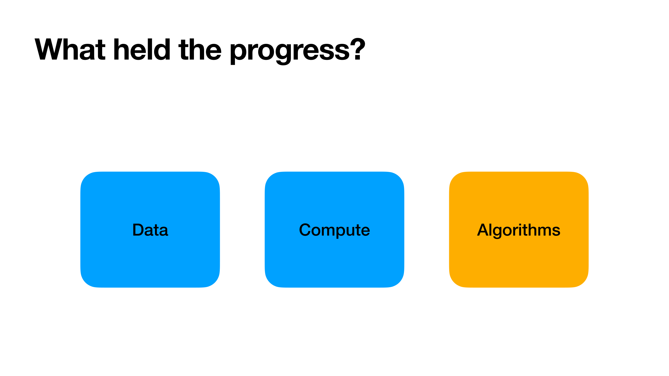
What held the progress?
Ways to compute derivatives
Problem formulation, symbolic differentiation, and finite differences
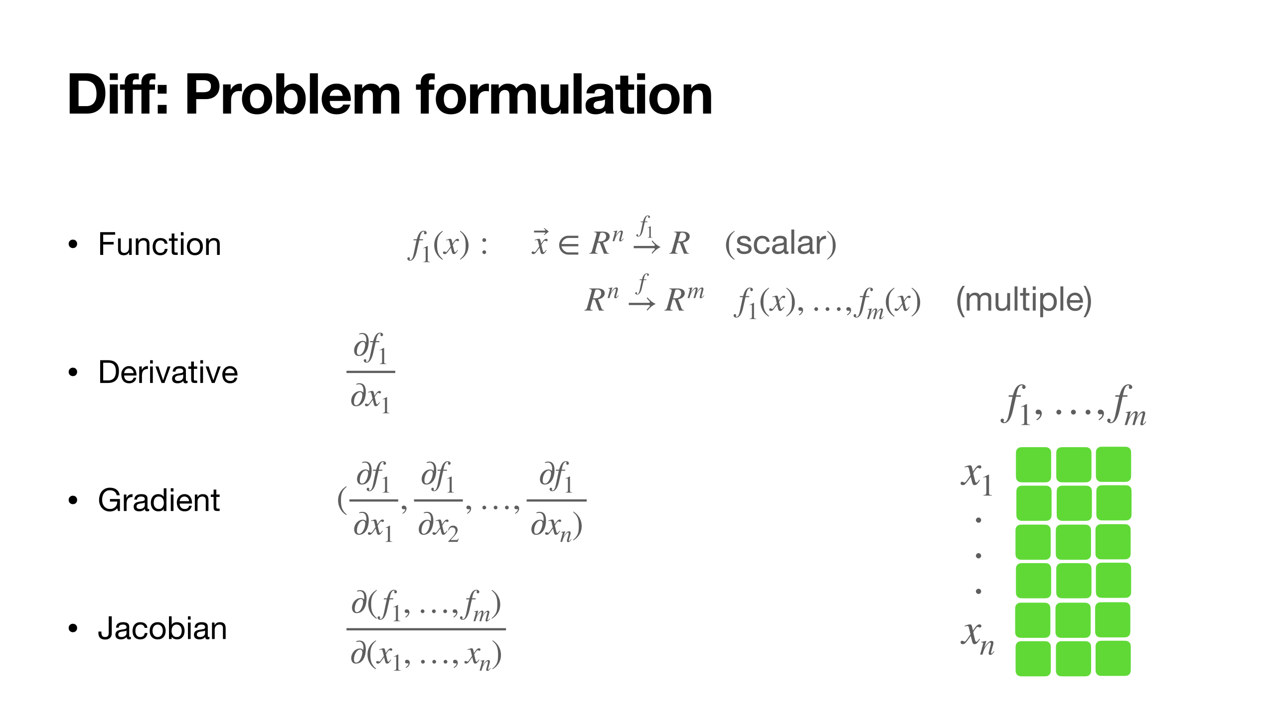
Diff: Problem formulation
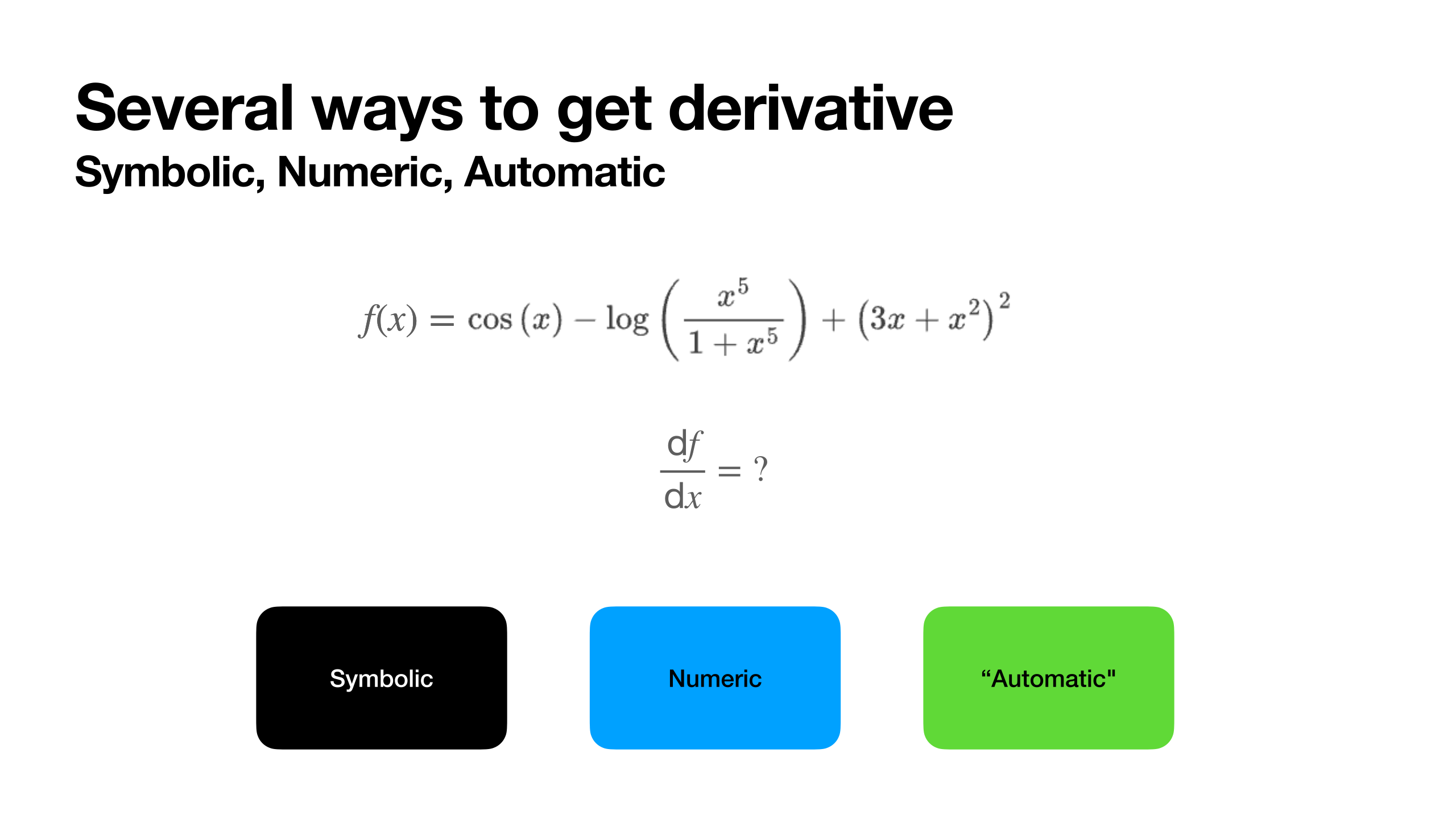
Several ways to get derivative
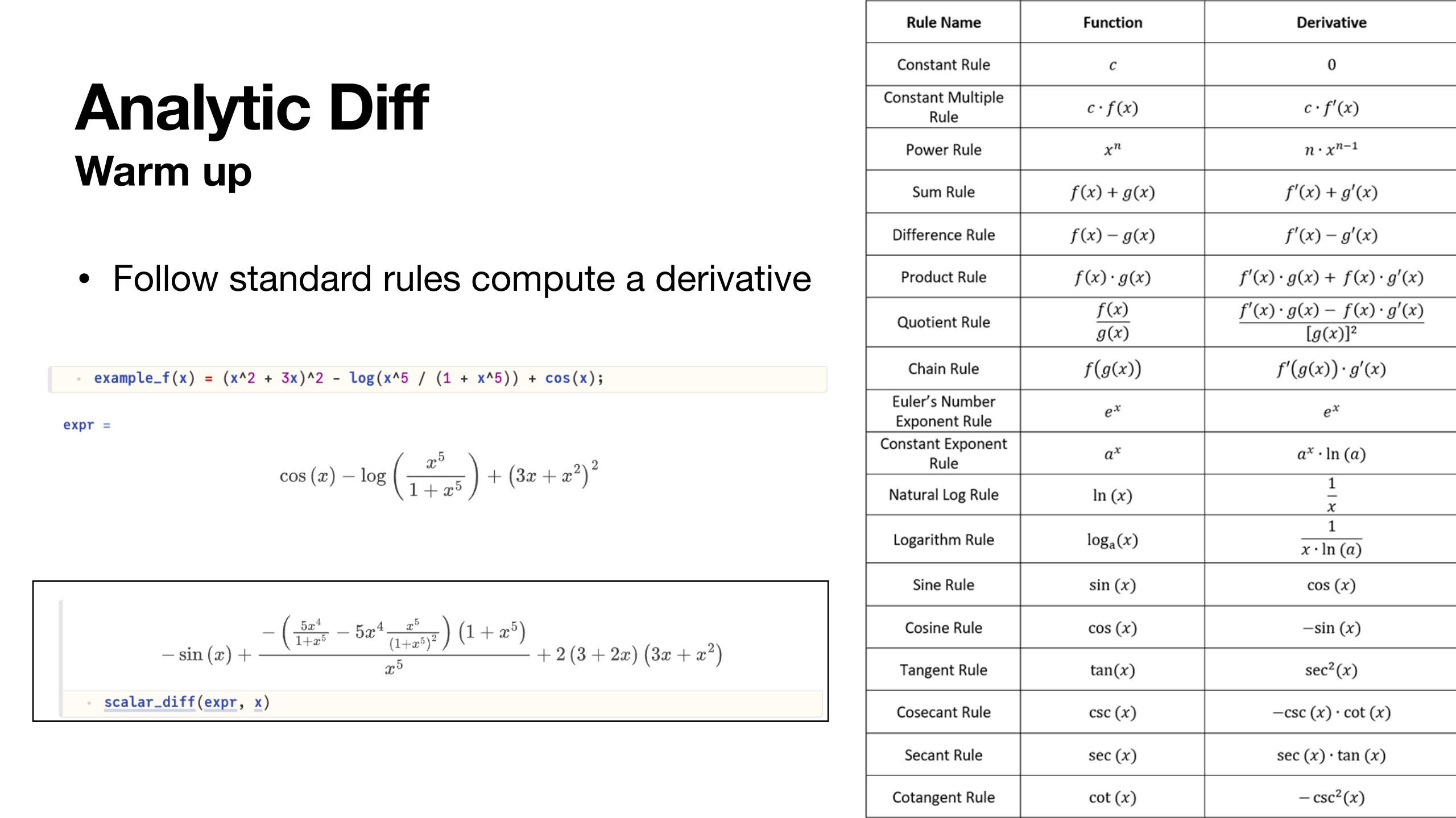
Analytic Diff
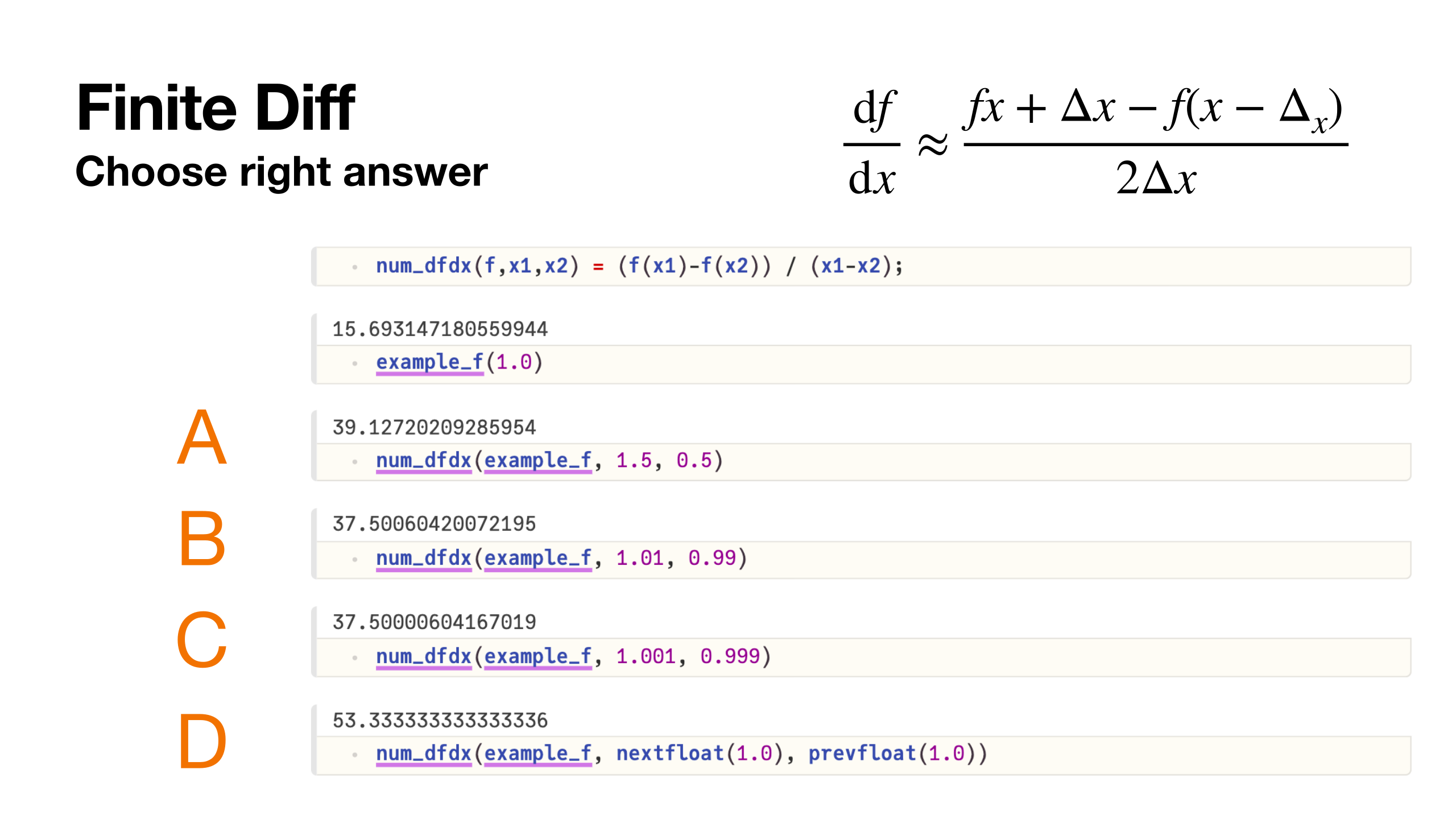
Finite Diff
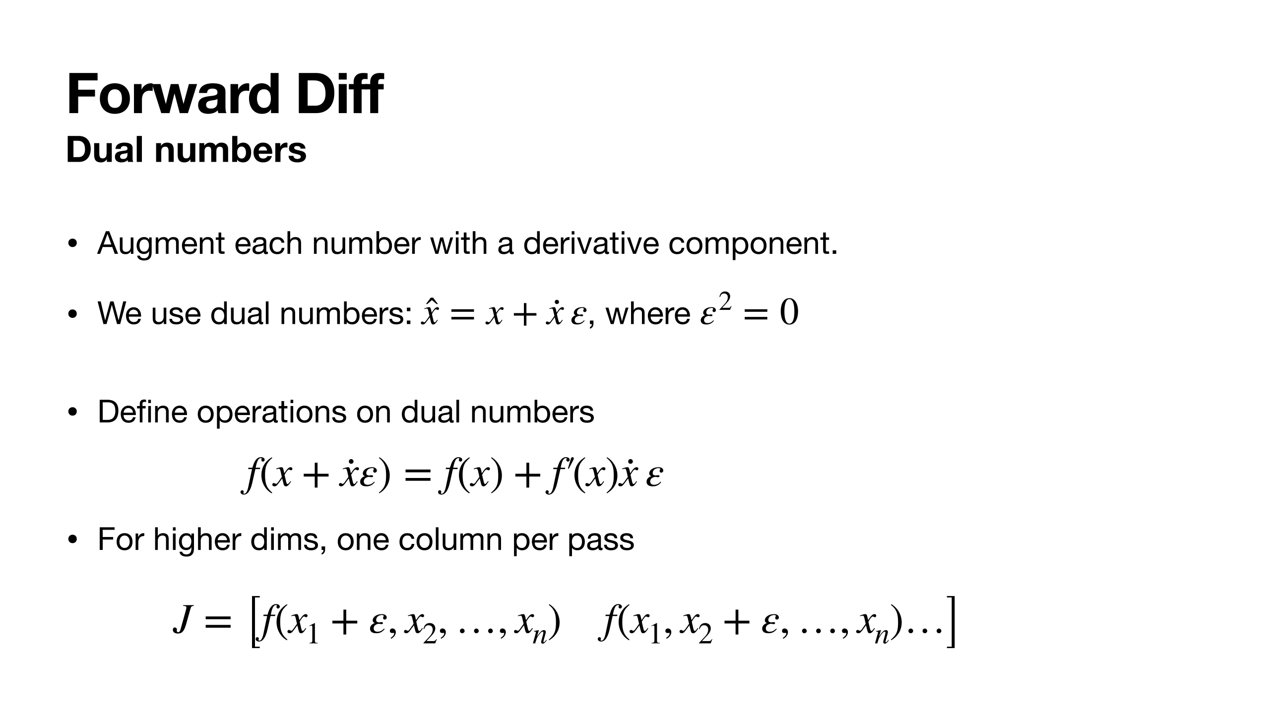
Forward mode
Propagate values and derivative components together
Forward Diff
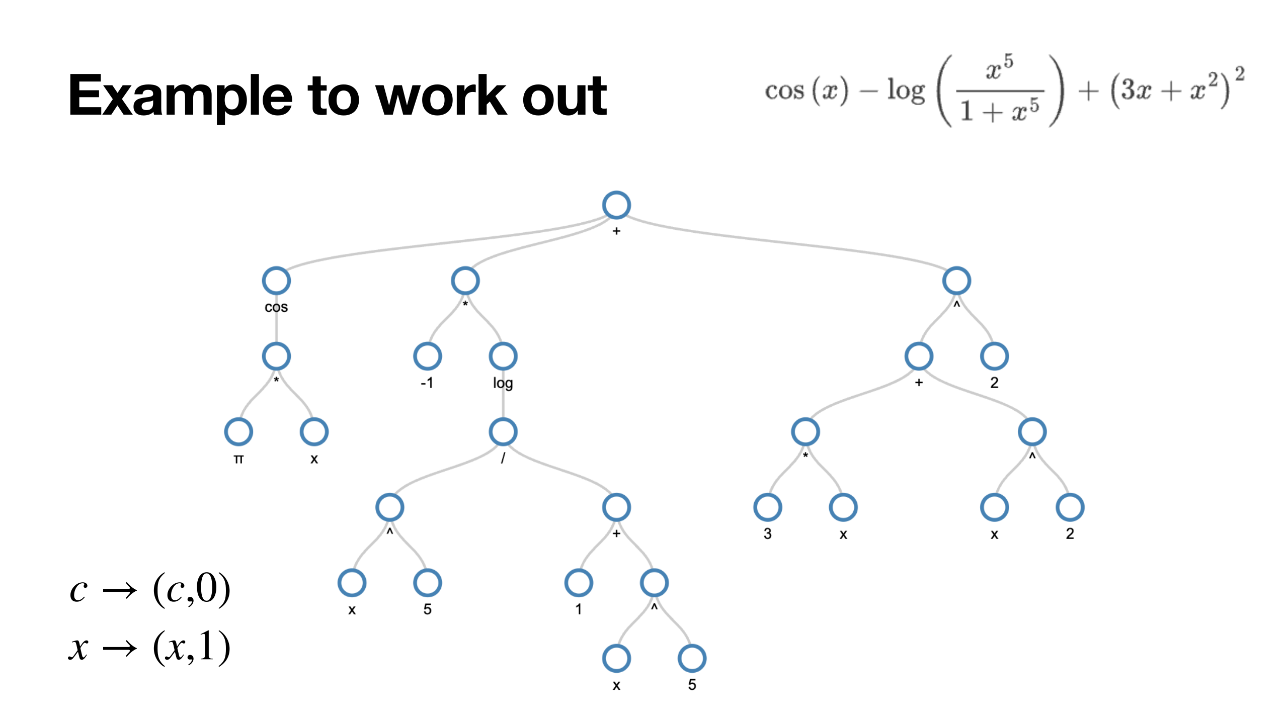
Example to work out
Reverse mode and backpropagation
Evaluate forwards, then propagate sensitivities backwards
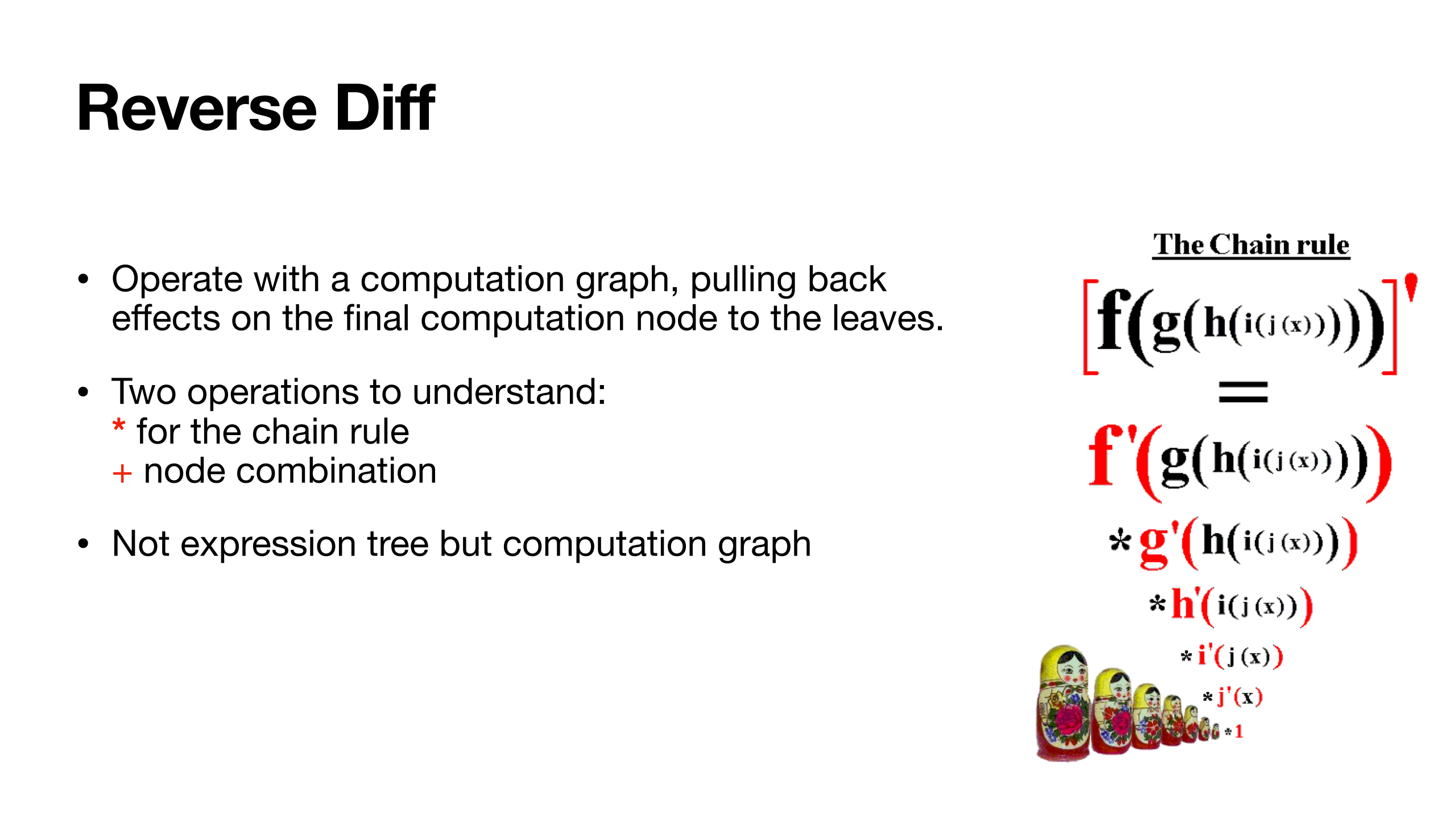
Reverse Diff
Backpropagation, step by step
We want the derivative of one loss with respect to every parameter.
Evaluate the program forwards and retain the values needed for derivatives.
Then propagate sensitivities backwards, using one local derivative at a time.
We will compute every step by hand before running the demonstration.
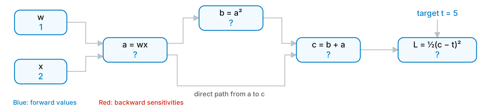
One graph, two paths
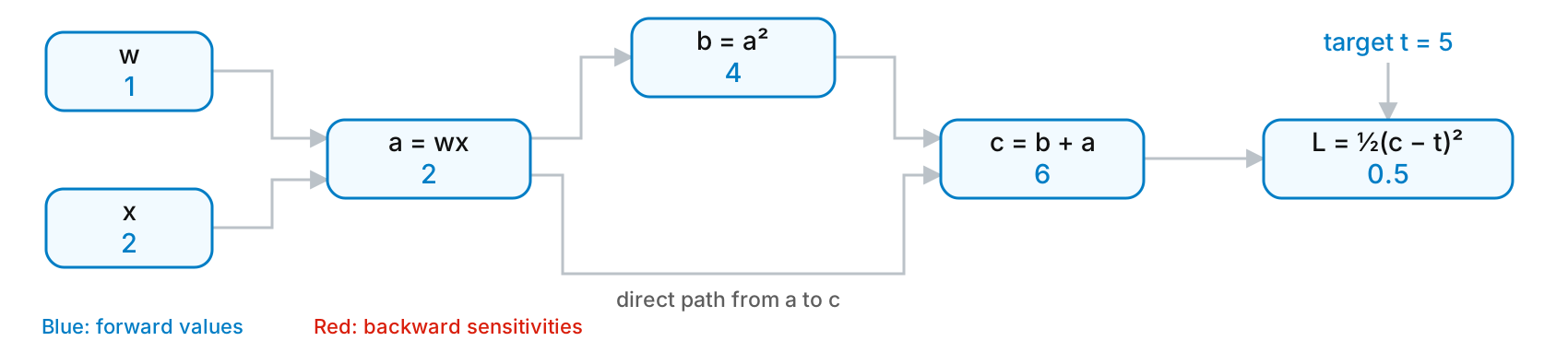
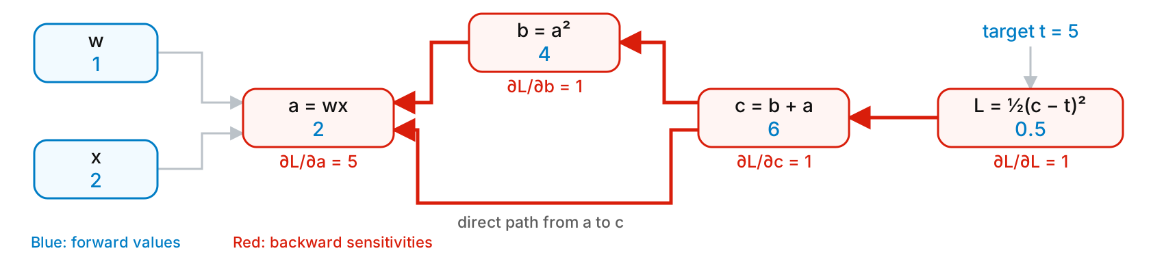
![Computation graph: w and x feed a=wx; a feeds b=a squared and c=b+a; c feeds the loss. The target t also feeds the loss.]()
The value affects the loss through two paths.
We train . The input and target stay fixed.
1. Forward pass
Start with , , and .
![Forward values: a=2, b=4, c=6, loss=0.5.]()
Keep the intermediate values. The backward pass will use them.
2. What travels backwards?
The adjoint of an intermediate is its sensitivity:
For a small perturbation, .
Forward value
“What number did this operation produce?”
Backward sensitivity
“How does this number affect the loss?”
Local backward rules
For an incoming sensitivity :
Addition
Send the sensitivity to both inputs.
Multiplication
Use the other input’s forward value.
Squaring
Use the local slope at the stored value.
The notation means add this contribution to the adjoint.
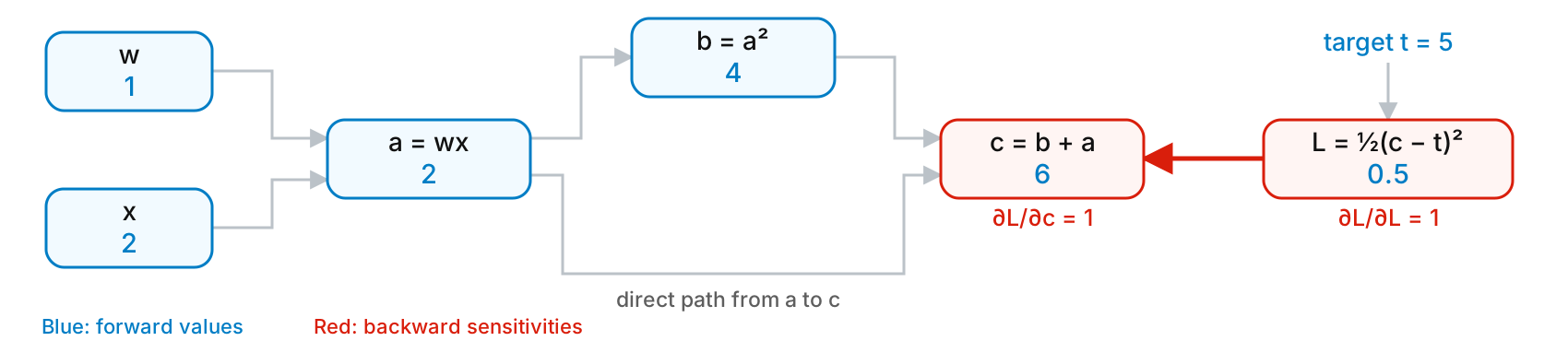
3. Backwards through the loss
![The reverse pass starts at loss with adjoint one and produces c adjoint one.]()
At this point, increasing slightly would increase the loss.
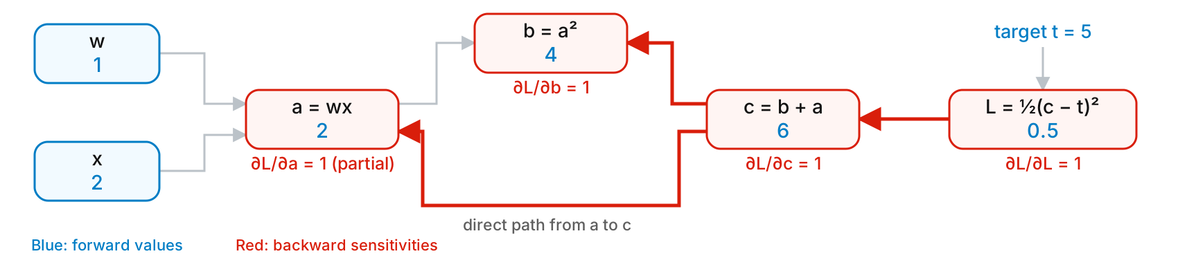
4. Backwards through the sum
![The addition sends adjoint one to b and a. The a adjoint is not complete yet.]()
This is only the direct-path contribution to .
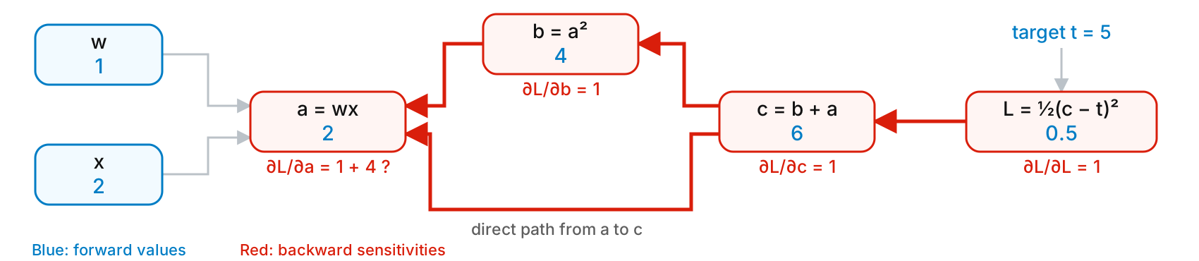
5. Backwards through the square
![The squared path contributes 2a times b adjoint = four to a.]()
Is now 1, 4, or 5?
6. Accumulation at a shared node
![Both reverse paths meet at a, giving total sensitivity five.]()
Multiply derivatives along each path. Add contributions from different paths.
Only propagate further once all contributions to the node have arrived.
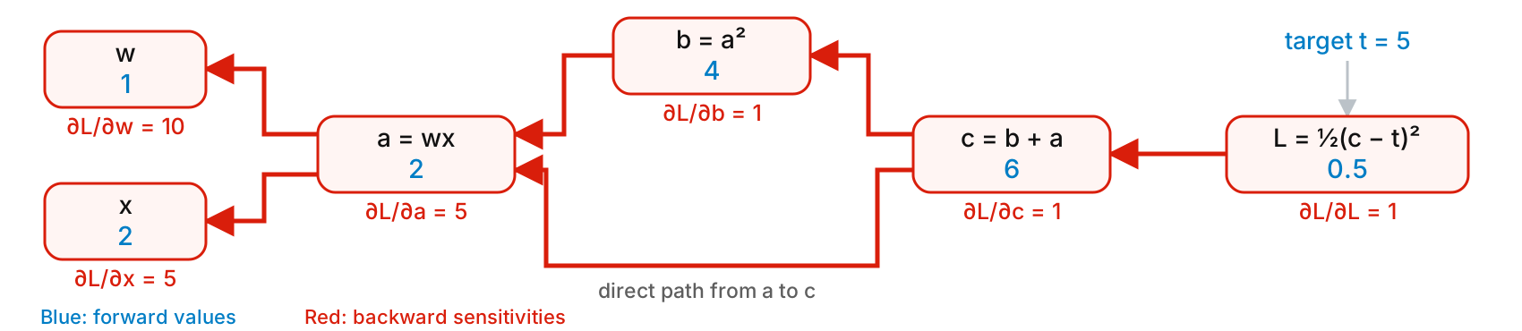
7. Backwards to the parameter
![Backpropagation through multiplication gives w adjoint ten and x adjoint five.]()
The derivative with respect to the trainable parameter is . We can also compute , even though is fixed during this update.
8. A parameter update
Backpropagation has finished. Now apply gradient descent with .
| Parameter |
1 |
0.9 |
| Prediction |
6 |
5.04 |
| Loss |
0.5 |
0.0008 |
The new loss requires a new forward pass. A larger step may increase it.
A neuron uses the same rules
Work backwards, starting at the scalar loss:
For a sigmoid, : reuse the activation from the forward pass.
Backpropagation through layers
Given the incoming sensitivity :
Repeat for the previous layer. Here denotes elementwise multiplication.
The reverse sweep in code
# Forward: record operations and their needed input values.
value = evaluate_in_dependency_order(graph)

# Backward: start with zero contributions everywhere.
adjoint = {node: 0.0 for node in graph}
adjoint[loss] = 1.0

for node in reversed(dependency_order):
    for input_edge in node.input_edges:
        parent = input_edge.source
        adjoint[parent] += (
            adjoint[node] * local_derivative(input_edge, value)
        )
Process edges, including repeated inputs. For , both edges contribute.
Checking a gradient
For our example, compute an independent central finite difference:
At , , , and :
Use this as a diagnostic on a small, smooth example.
Very small finite-difference steps amplify roundoff. At a nondifferentiable point, the comparison needs special care.
One reverse pass, many parameters
For one scalar loss, the reverse sweep computes all parameter derivatives.
Each operation sends sensitivities to its inputs. The work scales with the computation graph, with a constant-factor overhead for standard operations.
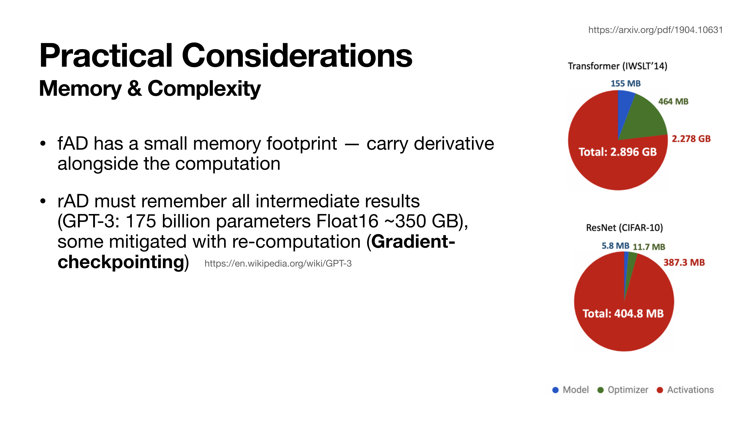
The tradeoff is memory: backward rules need values from the forward pass.
Checkpointing saves selected values and recomputes others.
Backpropagation demonstration
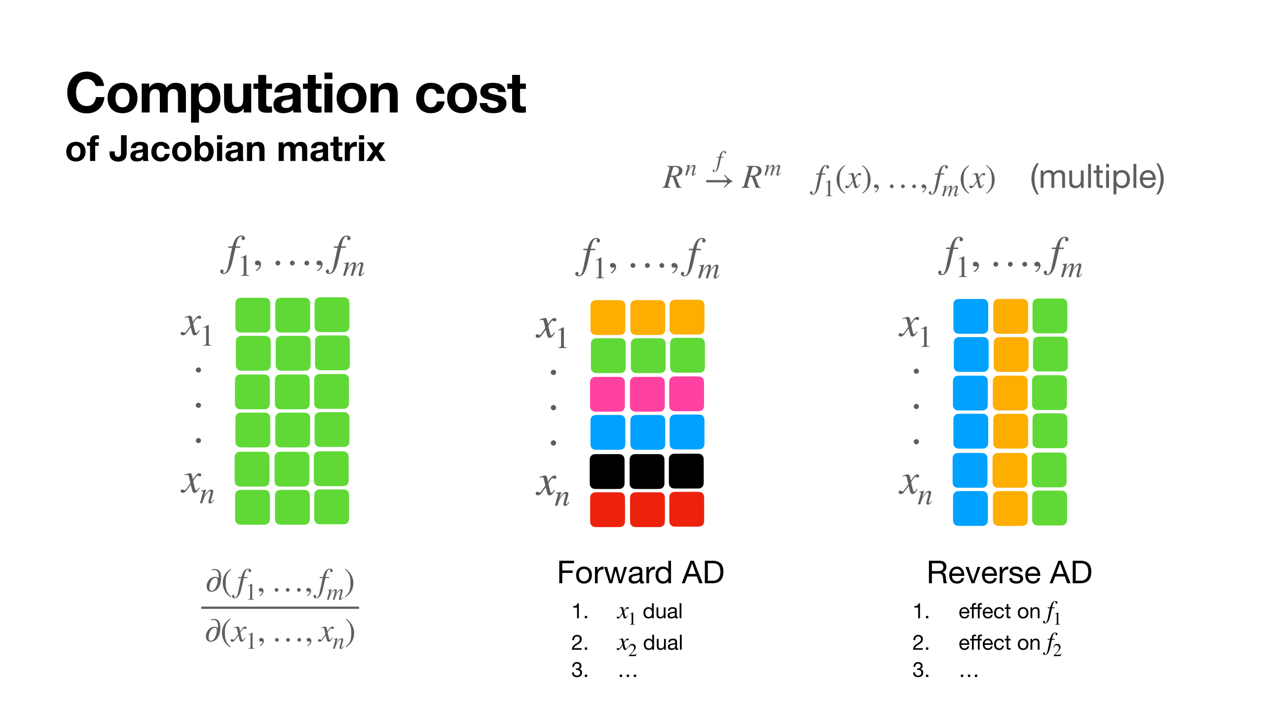
Computation cost
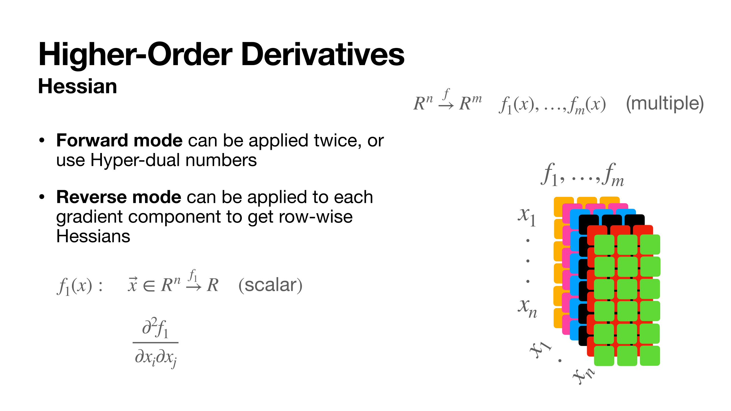
Higher-Order Derivatives
Practical Considerations
Automatic differentiation in practice
Frameworks, transformations, compilers, and implementation trade-offs
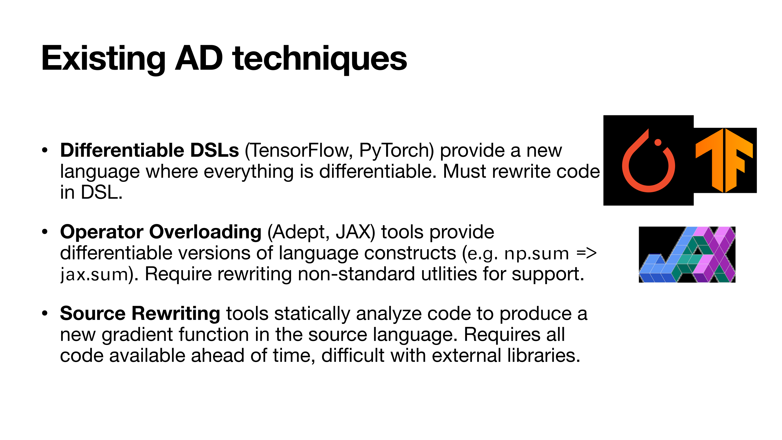
Existing AD techniques
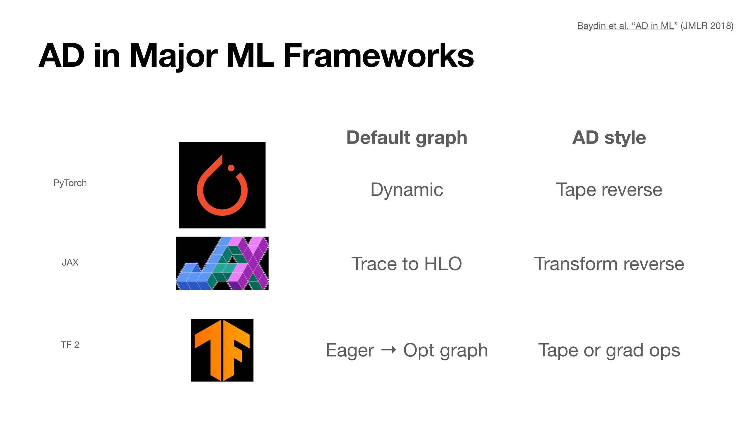
AD in Major ML Frameworks
Python ecosystem
| NumPy / SciPy |
Numerical arrays and scientific algorithms |
Derivatives supplied separately or approximated |
| SymPy |
Symbolic expressions |
diff(expression, variable) |
| JAX |
Array programs and function transformations |
jvp, vjp, grad |
| PyTorch |
Tensors, neural networks, training |
torch.func, .backward() |
| TensorFlow |
Tensors, models, training |
ForwardAccumulator, GradientTape |
| marimo |
Reactive Python notebooks |
Runs the chosen library’s code |
Forward evaluation and forward-mode AD
For , ordinary evaluation computes .
Forward-mode AD also propagates an input direction :
Tangent
A Jacobian-vector product (JVP) answers: how does the output change along this input direction?
Reverse mode: an output sensitivity
Evaluate , then choose an output sensitivity .
y, pullback = jax.vjp(F, x)
(sensitivity_x,) = pullback(u)
The pullback maps an output sensitivity back to the inputs.
For a scalar loss, seed the output with to obtain its gradient.
JVP: a direction through the inputs. VJP: a weighted combination of output sensitivities.
JAX: the lecture’s scalar loss
import jax
jax.config.update("jax_enable_x64", True)

def loss(w):
    a = 2.0 * w
    return 0.5 * (a**2 + a - 5.0)**2

value, tangent = jax.jvp(loss, (1.0,), (1.0,))
value, pullback = jax.vjp(loss, 1.0)
(gradient,) = pullback(1.0)

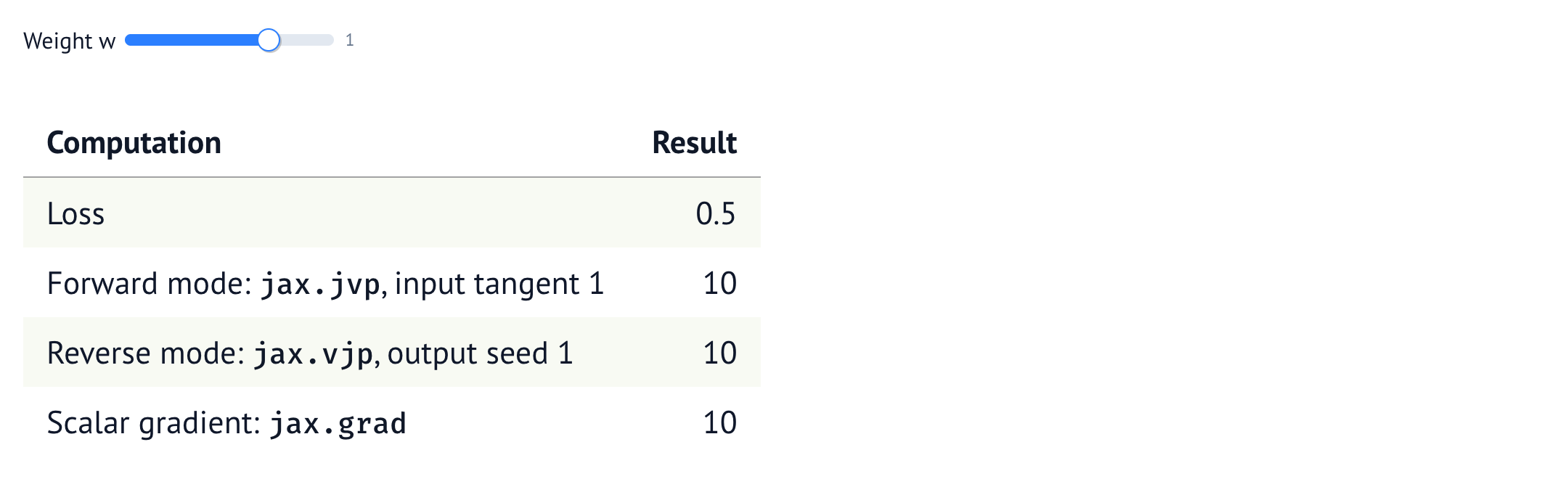
print(value, tangent, gradient)   # 0.5, 10.0, 10.0
print(jax.grad(loss)(1.0))        # 10.0
The input direction is . The scalar-loss output seed is also .
marimo: compare the two modes
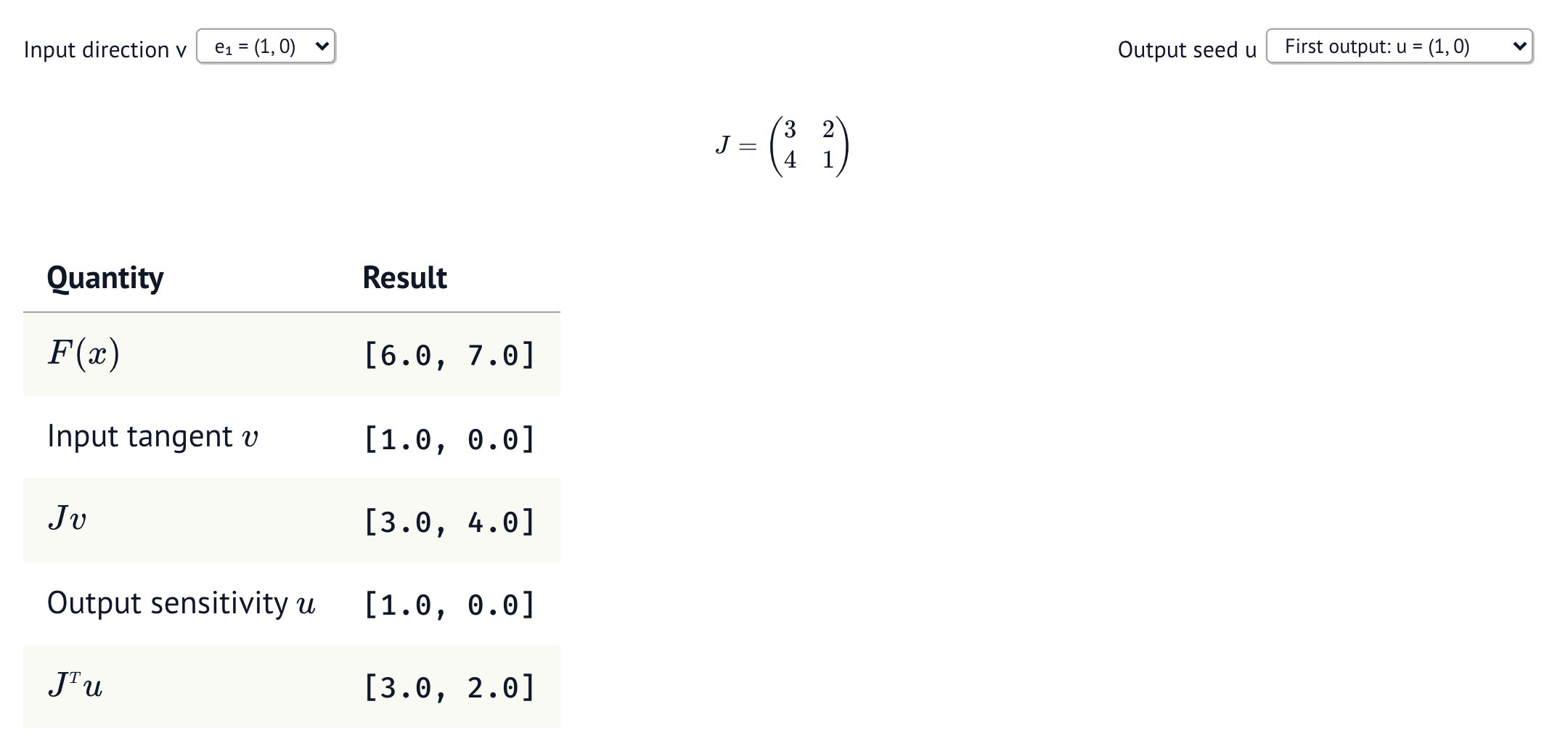
![Executed marimo notebook comparing loss 0.5 and derivative 10 using JAX jvp, vjp, and grad.]()
Change from to : predict the loss and gradient before rerunning.
A vector function
Forward: select a column
Reverse: select a row
For general seeds, compute linear combinations of columns or rows.
JAX: products and full Jacobians
import jax.numpy as jnp

def F(x):
    return jnp.array([x[0] * x[1], x[0]**2 + x[1]])

x = jnp.array([2.0, 3.0])
seed = jnp.array([1.0, 0.0])
y, Jv = jax.jvp(F, (x,), (seed,))  # [3., 4.]
y, pullback = jax.vjp(F, x)
(JTu,) = pullback(seed)            # [3., 2.]

J_forward = jax.jacfwd(F)(x)       # [[3., 2.],
J_reverse = jax.jacrev(F)(x)       #  [4., 1.]]
Both Jacobian functions return the same matrix. JVP and VJP need not build it.
marimo: input direction and output seed
![Executed marimo vector example with Jacobian [[3,2],[4,1]], JVP [3,4], and VJP [3,2].]()
Switch each seed to . Which column or row should appear?
PyTorch: a training step
w = torch.tensor(1.0, dtype=torch.float64, requires_grad=True)
optimizer = torch.optim.SGD([w], lr=0.01)

optimizer.zero_grad(set_to_none=True)
value = loss(w)                 # forward evaluation: 0.5
value.backward()               # reverse mode
print(w.grad.item())           # 10.0

optimizer.step()               # optimizer changes w
print(w.item())                # 0.9
print(loss(w).item())          # approximately 0.0008
.backward() accumulates into .grad. Clear gradients before the next step.
marimo: one optimizer step
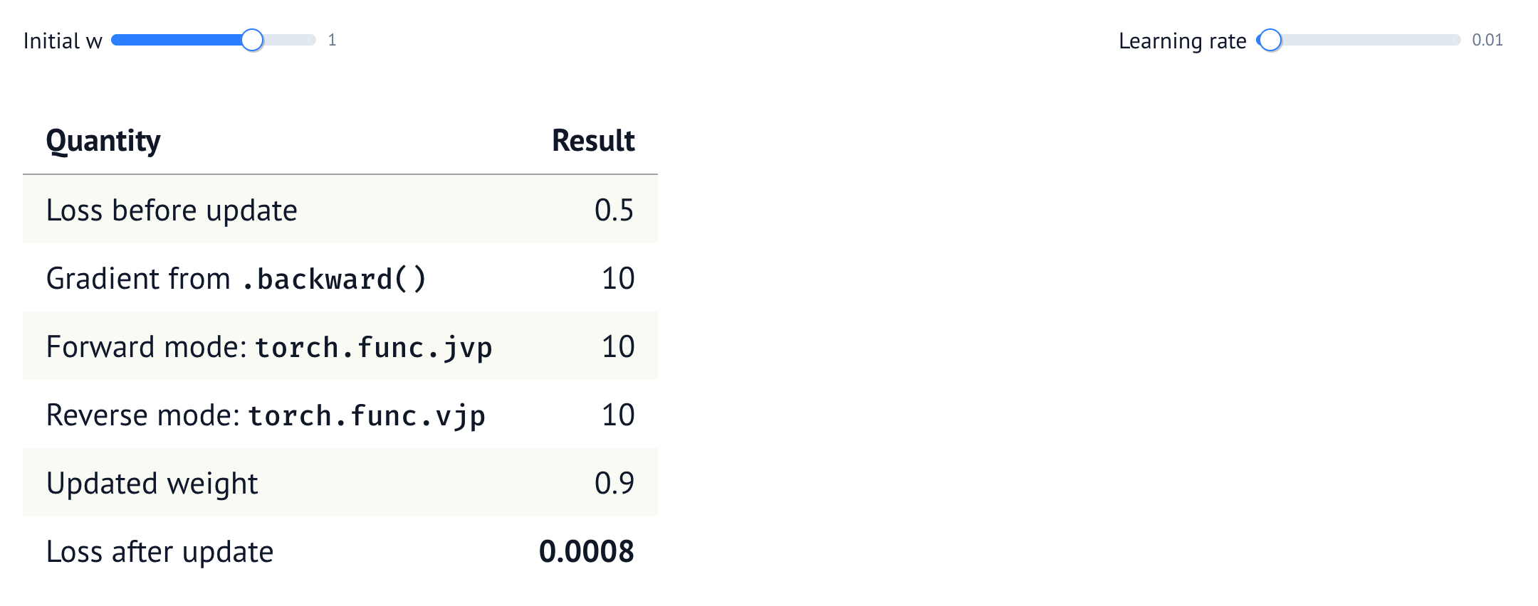
![Executed marimo PyTorch notebook: gradient ten, updated weight 0.9, loss decreases from 0.5 to 0.0008.]()
Increase the learning rate to . The gradient is still correct. What happens to the loss?
Choosing and checking an AD mode
For , think about what derivative you need.
| One input direction |
JVP / forward mode |
| Scalar loss, many parameters |
Gradient / reverse mode |
| Full Jacobian, few inputs |
jacfwd |
| Full Jacobian, few outputs |
jacrev |
Keep operations inside the library’s differentiable computation. Convert to NumPy or Python numbers after computing the derivative.
Check small examples analytically or with finite differences, and benchmark the real workload.
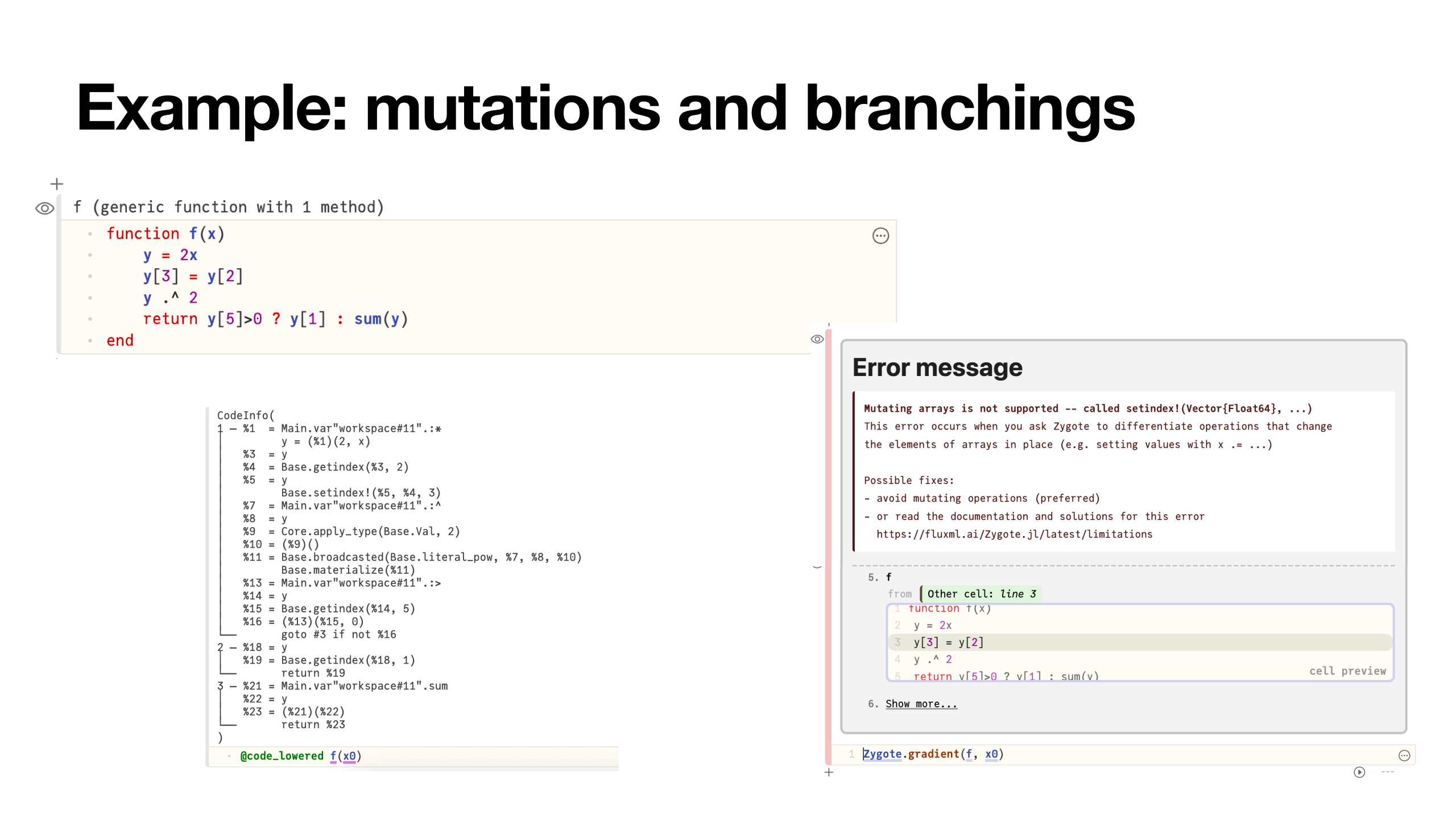
Example: mutations and branchings
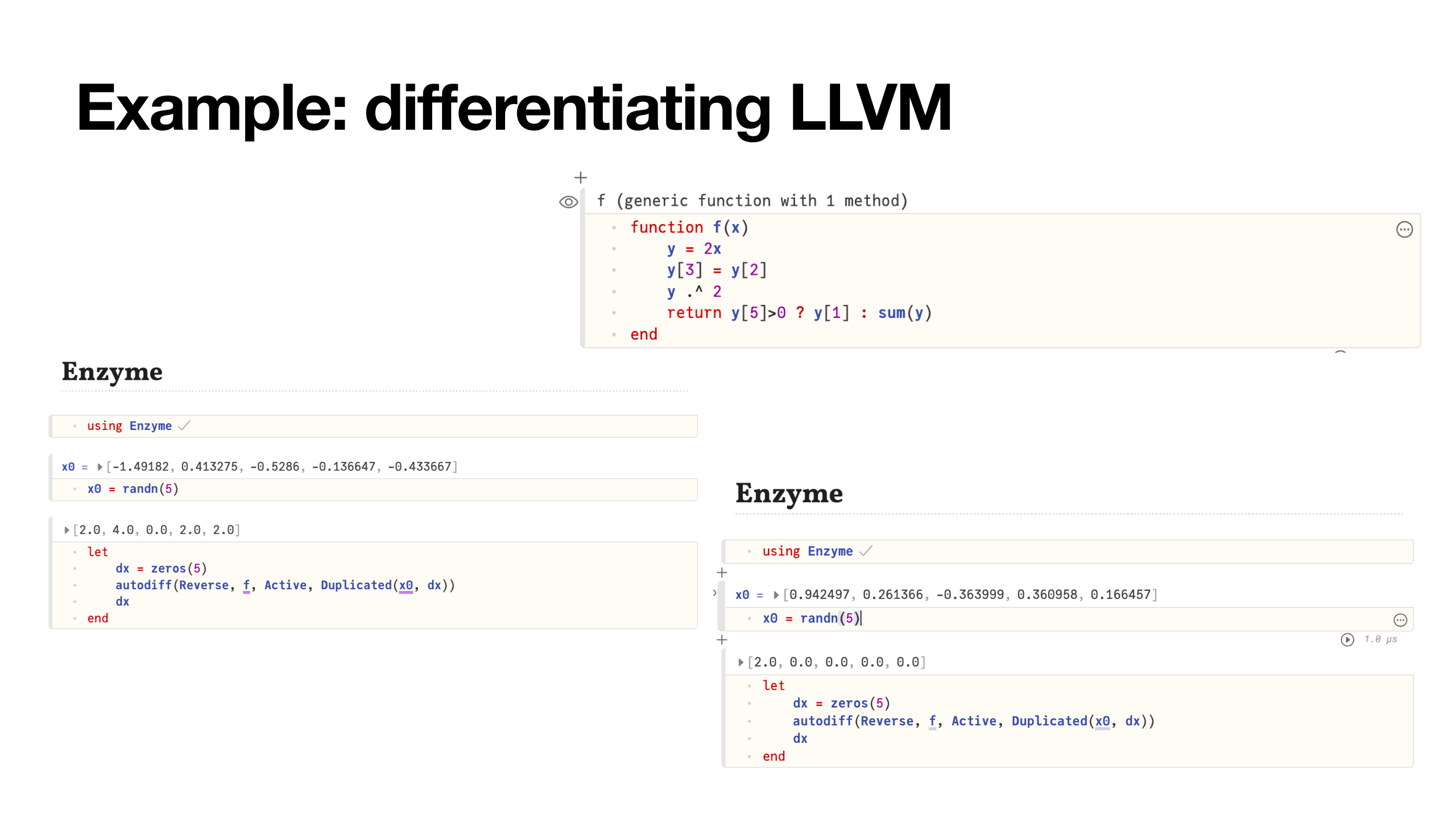
Example: differentiating LLVM
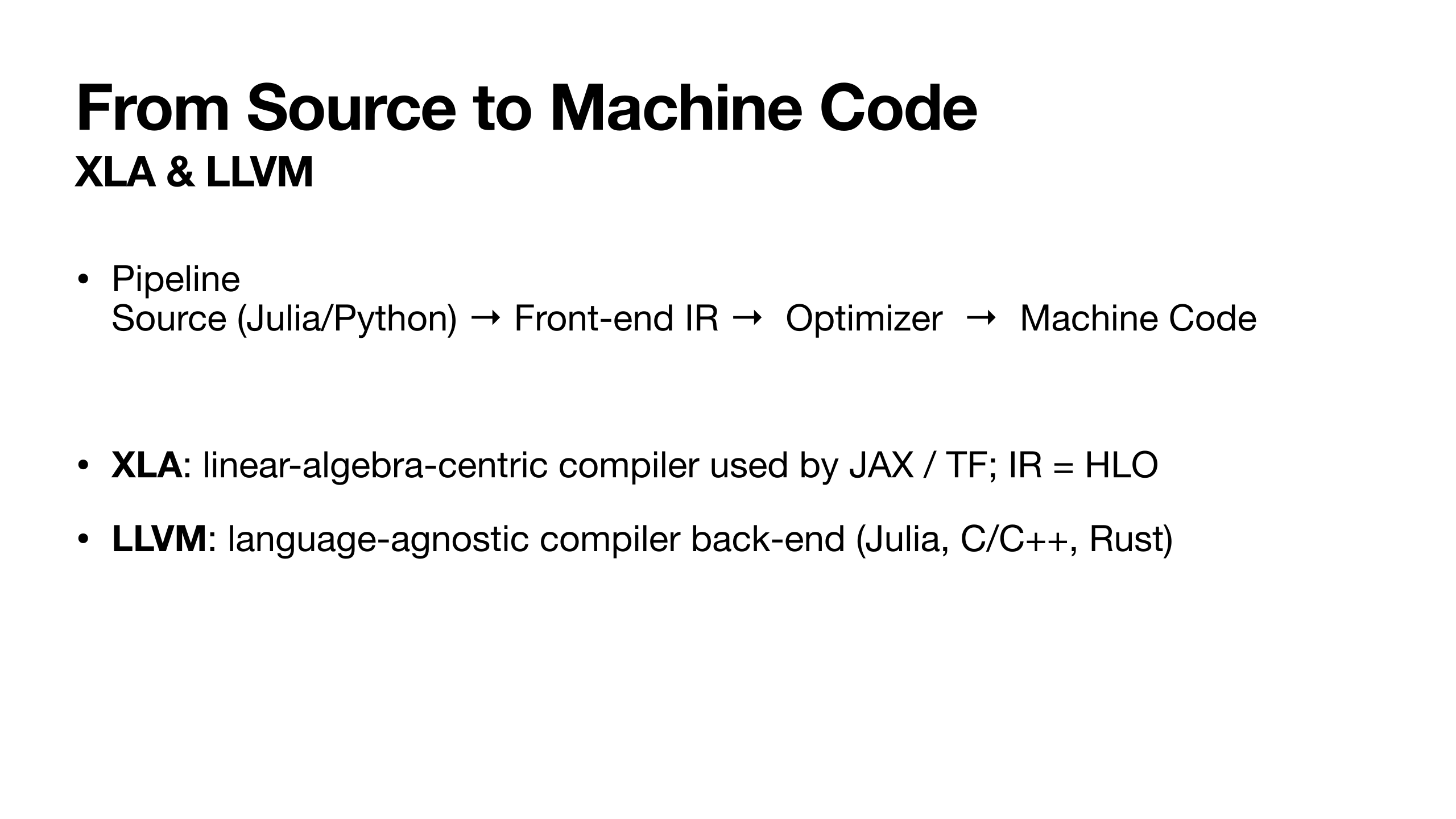
From Source to Machine Code
Historical and conceptual epilogue
An old algorithm, modern scale, and the cheap-gradient principle
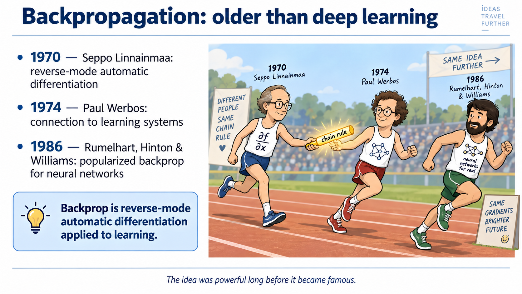
Backpropagation is older than deep learning
1970 — Seppo Linnainmaa
Systematic reverse accumulation for differentiating a program.
1974 — Paul Werbos
Connected backward differentiation with learning systems.
1986 — Rumelhart, Hinton & Williams
Demonstrated and popularized backpropagation for multilayer neural networks.
Backpropagation is reverse-mode automatic differentiation applied to a learning problem.
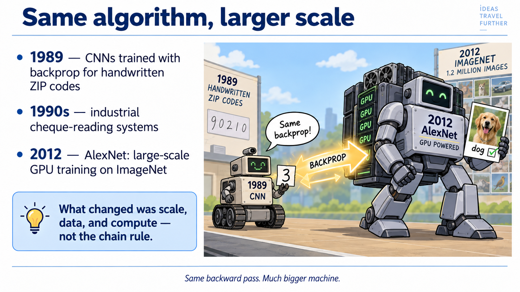
The same algorithm at larger scale
1989 — handwritten ZIP codes
LeCun and colleagues trained a convolutional network with backpropagation.
1990s — document recognition
Neural systems moved into deployed cheque and document processing.
2012 — AlexNet
GPU training, about 60 million parameters, and 1.2 million ImageNet training images.
Data, compute, architecture and scale changed dramatically. The chain rule did not.
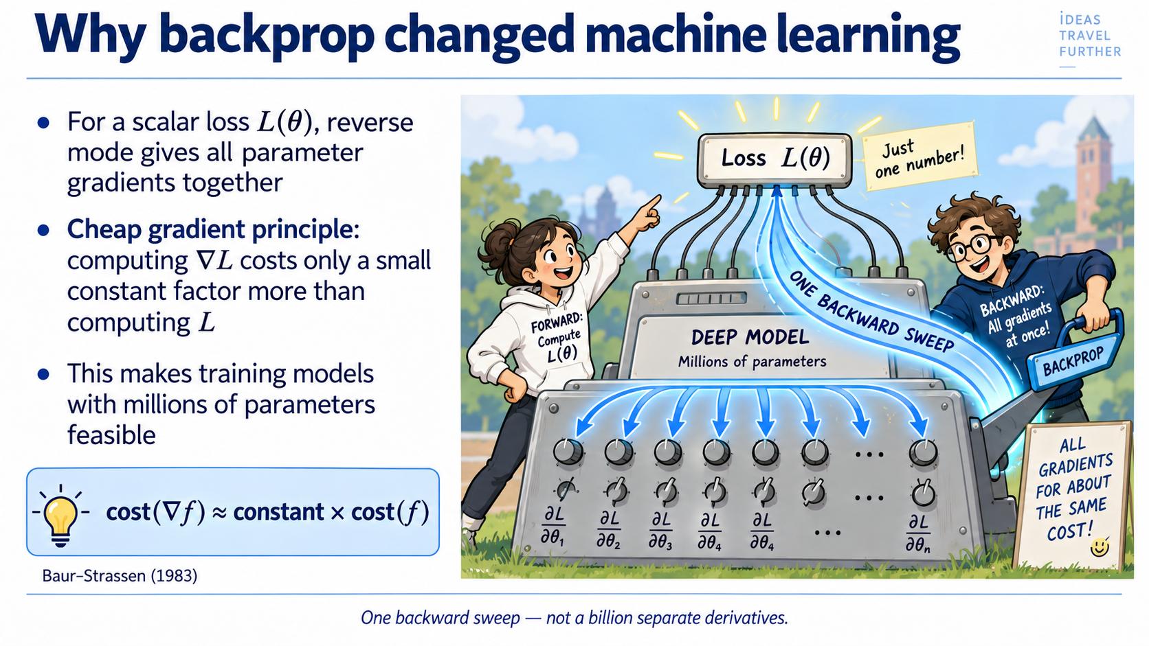
The surprising fact: gradients are cheap
For a scalar objective
one reverse sweep produces the complete gradient:
In practice, the backward pass costs a small constant multiple of the forward computation. It also needs stored or recomputed intermediate values.
or parameters do not require or separate derivative calculations.
EndBackup follows
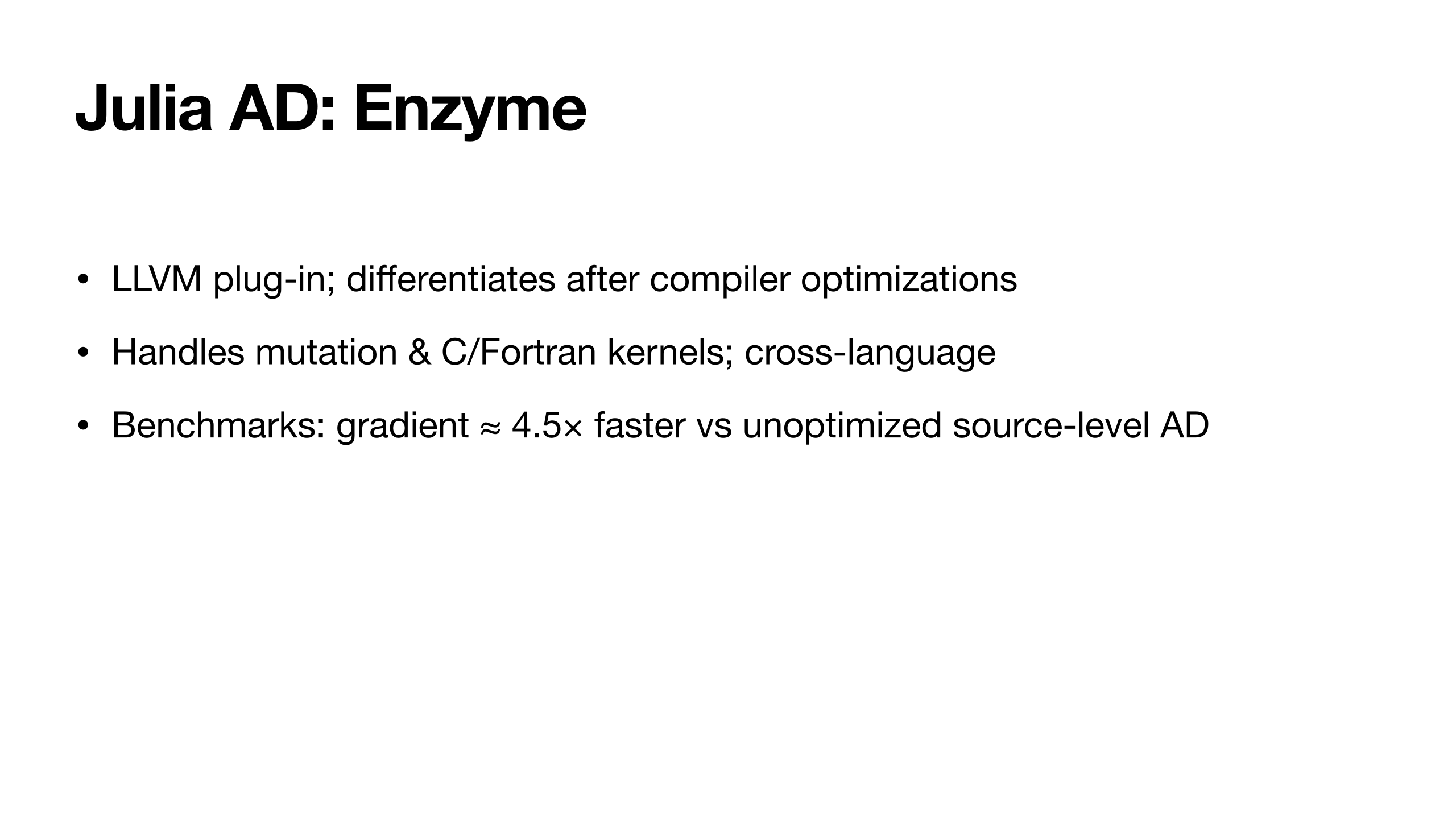
Julia AD: Enzyme
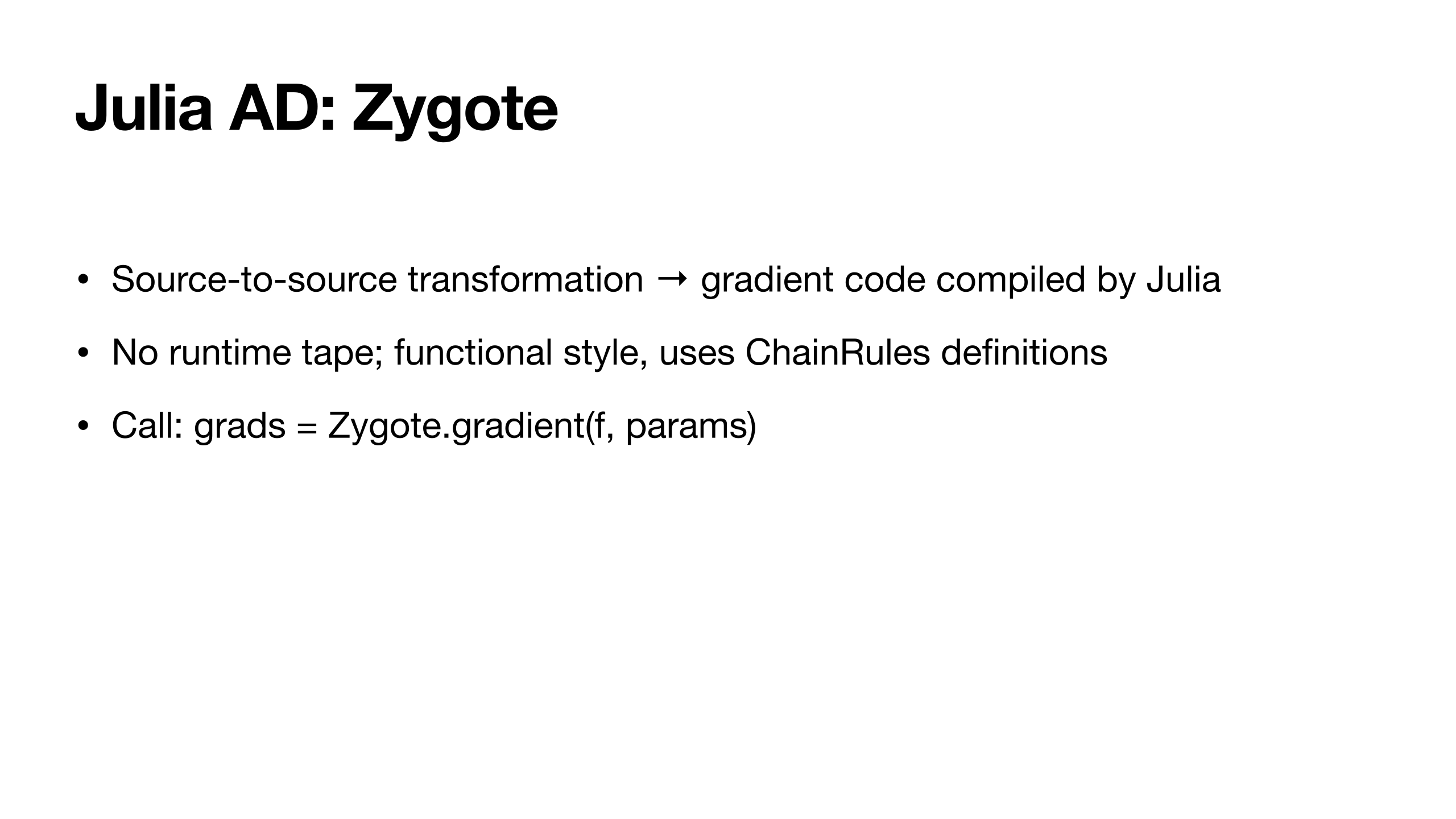
Julia AD: Zygote